Dynamo
╭━━━╮
╰╮╭╮┃
╱┃┃┃┣╮╱╭┳━╮╭━━┳╮╭┳━━╮
╱┃┃┃┃┃╱┃┃╭╮┫╭╮┃╰╯┃╭╮┃
╭╯╰╯┃╰━╯┃┃┃┃╭╮┃┃┃┃╰╯┃
╰━━━┻━╮╭┻╯╰┻╯╰┻┻┻┻━━╯
╱╱╱╱╭━╯┃
╱╱╱╱╰━━╯
Overview
Dynamo is built to be the Swiss-knife for price-movement & strength detection, it aims to provide a holistic view of the current price across multiple dimensions. This is achieved by combining 3 very specific indicators(RSI, Stochastic & ADX) into a single view. Each of which serve a different purpose, and collectively provide a simple, yet powerful tool to gauge the true nature of price-action.
Background
Dynamo uses 3 technical analysis tools in conjunction to provide better insights into price movement, they are briefly explained below:
Relative Strength Index(RSI)
RSI is a popular indicator that is often used to measure the velocity of price change & the intensity of directional moves. RSI computes the relative strength of the current price by comparing the security’s bullish strength versus bearish strength for a given period, i.e. by comparing average gain to average loss.
It is a range bound(0-100) variable that generates a bullish reading if average gain is higher, and a bullish reading if average loss is higher. Values over 50 are generally considered bullish & values less than 50 indicate a bearish market. Values over 70 indicate an overbought condition, and values below 30 indicate oversold condition.
Stochastic
Stochastic is an indicator that aims to measure the momentum in the market, by comparing most recent closing price of the security to its price range for a given period. It is based on the assumption that price tends to close near the recent high in an up trend, and it closes near the recent low during a down trend.
It is also range bound(0-100), values over 80 indicate overbought condition and values below 20 indicate oversold condition.
Average Directional Index(ADX)
ADX is an indicator that can quantify trend strength, it is derived from two underlying indices, known as Directional Movement Index(DMI). +DMI represents strength of the up trend, and -DMI represents strength of the down trend, and ADX is the average of the two.
ADX is non-directional or trend-neutral, which means, it does not follow the direction of the price, instead ADX will rise only when there is a strong trend, it does not matter if it’s an up trend or a down trend. Typical ranges of ADX are 25-50 for a strong trend, anything below 25 is considered as no trend or weak trend. ADX can frequently shoot upto higher values, but it generally finds exhaustion levels around the 60-75 range.
About the script
All these indicators are very powerful tools, but just like any other indicator they have their limitations. Stochastic & ADX can generate false signals in volatile markets, meaning price wouldn’t always follow through with what’s being indicated. ADX may even fail to generate a signal in less volatile markets, simply because it is based on moving averages, it tends to react slower to price changes. RSI can also lose it’s effectiveness when markets are trending strong, as it can stay in the overbought or oversold ranges for an extended period of time.
Dynamo aims to provide the trader with a much broader perspective by bringing together these contrasting indicators into a single simplified view. When Stochastic becomes less reliable in highly volatile conditions, one can cross validate their deduction by looking at RSI patterns. When RSI gets stuck in overbought or oversold range, one can refer to ADX to get better picture about the current trend. Similarly, various combinations of rules & setups can be formulated to get a more deterministic view, when working with either of these indicators.
There many possible use cases for a tool like this, and it totally depends on how you want to use it. An obvious option is to use it to trigger signals only after it has been confirmed by two or more indicators, for example, RSI & Stochastic make a great combination for cross-over or cross-under strategies. Some of the other options include trend detection, strength detection, reversals or price rejection points, possible duration of a trend, and all of these can very easily be translated into effective entry and exit points for trades.
How to use it
Dynamo is an easy-to-use tool, just add it to your chart and you’re good to start with your market analysis. Output consists of three overlapping plots, each of which tackle price movement from a slightly different angle.
Stochastic: A momentum indicator that plots the current closing price in relation to the price-range over a given period of time.
Can be used to detect the direction of the price movement, potential reversals, or duration of an up/down move.
Plotted as grey coloured histograms in the background.
Relative Strength Index(RSI): RSI is also a momentum indicator that measures the velocity with which the price changes.
Can be used to detect the speed of the price movement, RSI divergences can be a nice way to detect directional changes.
Plotted as an aqua coloured line.
Average Directional Index(ADX): ADX is an indicator that is used to measure the strength of the current trend.
Can be used to measure how strong the price movement is, both up and down, or to establish long terms trends.
Plotted as an orange coloured line.
Features
Provides a well-rounded view of the market movement by amalgamating some of the best strength indicators, helping traders make better informed decisions with minimal effort.
Simplistic plots that aim to convey clean signals, as a result, reducing clutter on the chart, and hopefully in the trader's head too.
Combines different types of indicators into a single view, which leads to an optimised use of the precious screen real-estate.
Final Note
Dynamo is designed to be minimalistic in functionality and in appearance, as it is being built to be a general purpose tool that is not only beginner friendly, but can also be highly-configurable to meet the needs of pro traders.
Thresholds & default values for the indicators are only suggestions based on industry standards, they may not be an exact match for all markets & conditions. Hence, it is advisable for the user to test & adjust these values according their securities and trading styles.
The chart highlights one of many possible setups using this tool, and it can used to create various types of setups & strategies, but it is also worth noting that the usability & the effectiveness of this tool also depends on the user’s understanding & interpretation of the underlying indicators.
Lastly, this tool is only an indicator and should only be perceived that way. It does not guarantee anything, and the user should do their own research before committing to trades based on any indicator.
Cari dalam skrip untuk "relative strength"

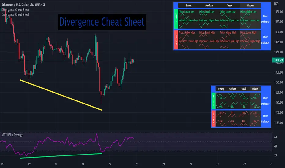
Divergence Cheat Sheet'Divergence Cheat Sheet' helps in understanding what to look for when identifying divergences between price and an indicator. The strength of a divergence can be strong, medium, or weak. Divergences are always most effective when references prior peaks and on higher time frames. The most common indicators to identify divergences with are the Relative Strength Index (RSI) and the Moving average convergence divergence (MACD).
Regular Bull Divergence: Indicates underlying strength. Bears are exhausted. Warning of a possible trend direction change from a downtrend to an uptrend.
Hidden Bull Divergence: Indicates underlying strength. Good entry or re-entry. This occurs during retracements in an uptrend. Nice to see during the price retest of previous lows. “Buy the dips."
Regular Bear Divergence: Indicates underlying weakness. The bulls are exhausted. Warning of a possible trend direction change from an uptrend to a downtrend.
Hidden Bear Divergence: Indicates underlying weakness. Found during retracements in a downtrend. Nice to see during price retests of previous highs. “Sell the rallies.”
Divergences can have different strengths.
Strong Bull Divergence
Price: Lower Low
Indicator: Higher Low
Medium Bull Divergence
Price: Equal Low
Indicator: Higher Low
Weak Bull Divergence
Price: Lower Low
Indicator: Equal Low
Hidden Bull Divergence
Price: Higher Low
Indicator: Higher Low
Strong Bear Divergence
Price: Higher High
Indicator: Lower High
Medium Bear Divergence
Price: Equal High
Indicator: Lower High
Weak Bear Divergence
Price: Higher High
Indicator: Equal High
Hidden Bull Divergence
Price: Lower High
Indicator: Higher High
Probabilistic Trend IndicatorAn indicator which attempts to assert the probability of the trend based on a given Sample Size and Look-Back Confirmation Size.
The green dots indicate the probability given to price.
The orange dots indicate the probability given to volume.
The aqua line is a weighted average between them.
The Sample Size is the number of candles to include in the entire calculation.
- This number should be higher to gather more data.
The Look-Back Confirmation Size is the number of candles to include, to confirm the current candles relative strength.
- This number should be lower to give a stronger closer relative reading.
Values above 50 indicate a strengthening position toward prices increasing.
- The strength of this value is weakly exponential and may max out around 80
Values below 50 indicate a strengthening position toward prices decreasing.
- The strength of this value is weakly exponential and may max out around 20
~ Enjoy!
Sentival | QuantEdgeBIntroducing Sentival by QuantEdgeB.
An Adaptive Multi-Factor Indicator for Market Valuation & Trend Strength
____
Overview
The Sentival Valuation System is a medium-term, multi-factor valuation tool designed to assess market conditions using a combination of momentum, mean reversion, and risk-adjusted metrics. It provides traders and investors with a dynamic score reflecting market valuation, ranging from strongly oversold to strongly overbought conditions.
This system leverages a diverse range of technical indicators, including momentum oscillators, volatility measures, risk ratios, and mean-reversion metrics, providing a holistic view of market conditions.
____
1. Key Features
🛠 Multi-Factor Valuation Model
Sentival aggregates nine different indicators, normalizing and rescaling them into a standardized z-score-based valuation system. The final output represents an average of the selected indicators, allowing for flexible customization based on the user’s preference.
📊 Customizable Indicator Selection
Users can enable or disable any of the nine valuation factors, ensuring the system adapts to different market environments, trading styles, and assets.
🔄 Multi-Timeframe Adaptability
Sentival can be used across different time horizons, making it suitable for short-term mean reversion, medium-term traders, or long-term valuation analysis by simply adjusting the timeframe and indicator settings. This flexibility allows traders to adapt Sentival to various market conditions and trading objectives.
🎨 Intuitive Dashboard & Color Coding
- Dynamic Heatmap & Dashboard: Displays valuation strength across multiple factors.
- Gradient-Based Overbought/Oversold Signals: Clear color-coded signals for easy interpretation.
- Background Highlighting: Optional oversold/overbought background zones.
🏆 Statistical & Risk-Based Insights
- Standardized Rescaling & Z-Score Analysis to prevent bias from individual indicators.
- Risk-Adjusted Metrics such as Sharpe, Sortino, and Omega Ratios help assess the overall market risk appetite.
- Trend Following Mode (TF Display): Users can enable the "Trend Following" option to display the trend direction, helping to align valuation signals with the broader market trend.
____
2. How It Works
Sentival is a multi-factor trend and momentum analysis system, designed to track market cycle shifts using a combination of volatility, momentum, risk assessment, and valuation mechanisms. Instead of focusing on one dimension of the market, Sentival integrates multiple methodologies to cross-validate signals and reduce noise. Each indicator in Sentival plays a specific role, ensuring confirmation across different market conditions.
How Each Component Works Together
1️⃣ Chande Momentum Oscillator (CMO)
• A momentum-based measure that determines whether price action is dominated by upward or downward forces.
• Works well in combination with volatility measures to confirm whether a move is sustainable.
2️⃣ Disparity Index
• Measures the distance between price and its moving average, acting as an overextension filter.
• Ensures that trend-following signals are not driven by short-term spikes but sustained trends.
3️⃣ Bollinger Bands % (BB%)
• A volatility measure that indicates how far price is from the statistical mean.
• Helps identify trend exhaustion points where price moves become unstable.
4️⃣ Relative Strength Index (RSI)
• A trend confirmation layer, ensuring that momentum strength aligns with price movement.
• Adds an additional check to prevent false breakouts.
5️⃣ Rate of Change (RoC)
• Captures the speed of price movement, ensuring that the market has enough momentum for trend continuation.
• Works well with risk indicators to filter weaker moves.
6️⃣ Price Z-Score
• A statistical tool to measure how far price is from its long-term equilibrium.
• Helps prevent entering overstretched trends too late.
7️⃣ Risk Ratios (Sharpe, Sortino, Omega)
• This is the risk-adjusted performance component, ensuring that trends have a healthy risk-reward balance.
• Helps determine when a trend has structurally strong backing rather than speculative movement.
8️⃣ Hurst Cycle Analysis
• Measures the persistence of trends by analyzing price fractals.
• Ensures that the market regime is either trending or mean-reverting, improving trade confidence.
9️⃣ Commodity Channel Index (CCI)
• Helps identify strong trend conditions, adding another layer of momentum confirmation.
• Works well with other oscillators to prevent misreading counter-trends.
🔗 Why These Components Work Well Together
• Momentum + Volatility + Risk → Instead of relying on a single category, Sentival merges multiple dimensions of market behavior into a cohesive signal.
• Filters Out False Signals → Combining momentum oscillators, volatility measures, and risk-adjusted metrics ensures high-confidence entries.
• Adaptability Across Market Regimes → Whether the market is trending, consolidating, or volatile, the system adjusts dynamically.
• Cross-Validation for Trend Strength → If multiple components align, it increases certainty that a trend is real and sustainable.
____
3. Sentival Scanner - table breakdown
The dashboard-style table generated is designed to give traders a holistic market view at a glance. It processes a variety of technical signals and distills them into readable labels, visual strength bars, and actionable trend states. Here's a breakdown of what each section means:
1. Direction
This section analyzes whether the average Z-score (a composite of several indicators) is increasing, decreasing, or neutral over time. It does this using a smoothed trend of the Z-score, comparing recent values to older ones.
2. Momentum
Momentum is derived from the rate of change (RoC) of the average Z-score. It evaluates how strong the current move is. If momentum is above a certain positive threshold, it’s considered positive, if below a negative threshold, it’s negative, otherwise it’s neutral.
3. Impulse
Impulse reflects the velocity of momentum — in other words, is the market speeding up or slowing down? High positive values suggest strong acceleration (strong impulse), while negative values show deceleration or stalling.
4. Drive
This metric combines momentum and velocity to create a descriptive phrase that captures the market’s behavior. For example:
• “Strong Upside” means strong momentum with acceleration.
• “Fading Downside” means bearish momentum losing steam.
• “Neutral” appears when momentum is indecisive.
5. Deviation Distance
This represents how far the market price is from fair value in terms of standard deviation units (σ). It’s calculated using Z-scores and classified as:
• +1σ, +2σ, etc., for overvalued regions.
• −1σ, −2σ, etc., for undervalued areas.
• “At Fair Value” if close to the mean.
6. Bull and Bear Strength Bars
The system computes both bullish and bearish strength, using distance from fair value, the rate of change, and the velocity. These strengths are displayed as progress bars, giving a quick visual cue of conviction. The table labels them as:
• “Bull Conviction” if there's a long bias.
• “Bull Potential” if bullish but undecided.
• “Bear Conviction” or “Bear Potential” for short-side equivalents.
7. Trend Signal
This is a simple label that tells you if the scanner recommends a Long, Short, or Cash (neutral) stance based on threshold logic. It is based on whether the average Z-score crosses above a long threshold or below a short one.
8. Stage
The “Stage” label summarizes the valuation environment based on the composite Z-score:
• Strong Undervalued
• Moderately Undervalued
• Fair Value
• Overvalued, etc.
This stage helps traders know whether they are operating in cheap or expensive territory statistically.
Summary
Overall, this table merges advanced technical signals like momentum, volatility, valuation, and risk into a digestible format that updates dynamically with each bar. The goal is to provide traders with a 360° perspective on market conditions, tailored for both trend-following and mean-reversion strategies.
___________
4. Sentival Valuation Score & Interpretation
🔹 Sentival Score Ranges
- 📉 Strongly Oversold (-2 and below) → Market is extremely undervalued; potential reversal.
- 📉 Moderately Oversold (-1.5 to -2) → Discounted market conditions, buying interest may emerge.
- 📉 Slightly Oversold (-0.5 to -1.5) → Possible accumulation phase.
- ⚖ Fair Value (-0.5 to +0.5) → Market trading at equilibrium.
- 📈 Slightly Overbought (+0.5 to +1.5) → Initial signs of market strength.
- 📈 Moderately Overbought (+1.5 to +2) → Market heating up, caution warranted, selling interest may emerge.
- 📈 Strongly Overbought (+2 and above) → Extreme valuation, increased risk of correction.
This classification helps traders gauge overall market sentiment and make better allocation decisions.
Note: Past valuations and buy/sell signals generated by Sentival do not guarantee future performance. Market conditions can change, and proper risk management should always be applied.
____
5. Use Cases & Applications
🔹 📊 Market Rotation & Asset Allocation
- Used as a valuation model to determine if a market or asset is undervalued or overvalued.
- Rotational strategies can benefit from the valuation score by switching exposure between assets.
🔹 📈 Medium-Term Trend Identification
- Detects overbought and oversold conditions while filtering out short-term noise.
- Can be combined with other trend-following indicators for confluence-based strategies.
🔹 🔄 Mean Reversion & Momentum Trading
- Provides statistical validation for momentum breakouts or mean reversion signals.
- Useful for long-short trading strategies, determining optimal entry & exit points.
____
Conclusion
Sentival is a powerful universal valuation system for traders and investors seeking a data-driven, multi-factor approach to market valuation. With its combination of momentum, trend, risk-adjusted, and mean-reversion indicators, it provides a robust, adaptable, and statistically sound framework for making informed market decisions.
🔹 Who Should Use Sentival?
✅ Swing Traders & Medium-Term Investors looking for structured valuation metrics.
✅ Quantitative & Systematic Traders incorporating multi-factor models.
✅ Portfolio Managers optimizing exposure to different market regimes.
🔹 Disclaimer: Past performance is not indicative of future results. No trading strategy can guarantee success in financial markets.
🔹 Strategic Advice: Always backtest, optimize, and align parameters with your trading objectives and risk tolerance before live trading.

RSI+Stoch Band Oscillator📈 RSI + Stochastic Band Oscillator
Overview:
The RSI + Stochastic Band Oscillator is a technical indicator that combines the strengths of both the Relative Strength Index (RSI) and the Stochastic Oscillator. Instead of using static thresholds, this indicator dynamically constructs upper and lower bands based on the RSI and Stochastic overbought/oversold zones. It then measures the relative position of the current price within this adaptive range, effectively producing a normalized oscillator.
Key Components:
RSI-Based Dynamic Bands:
Using RSI values and exponential moving averages of price changes, upper and lower dynamic bands are constructed.
These bands adjust based on overbought and oversold levels, offering a more responsive framework than fixed RSI thresholds.
Stochastic-Based Dynamic Bands:
Similarly, Stochastic %K and %D values are used to construct dynamic bands.
These adapt to overbought and oversold levels by recalculating potential high/low values within the lookback window.
Oscillator Calculation:
The oscillator (osc) is computed as the relative position of the current close within the combined upper and lower bands of both RSI and Stochastic.
This value is normalized between 0 and 100, allowing clear identification of extreme conditions.
Visual Features:
The oscillator is plotted as a line between 0 and 100.
Color-filled areas highlight when the oscillator enters extreme zones:
Above 100 with falling momentum: Red zone (potential reversal).
Below 0 with rising momentum: Green zone (potential reversal).
Additional trend conditions (falling/rising RSI, %K, and %D) are used to strengthen reversal signals by confirming momentum shifts.

Enhanced Fuzzy SMA Analyzer (Multi-Output Proxy) [FibonacciFlux]EFzSMA: Decode Trend Quality, Conviction & Risk Beyond Simple Averages
Stop Relying on Lagging Averages Alone. Gain a Multi-Dimensional Edge.
The Challenge: Simple Moving Averages (SMAs) tell you where the price was , but they fail to capture the true quality, conviction, and sustainability of a trend. Relying solely on price crossing an average often leads to chasing weak moves, getting caught in choppy markets, or missing critical signs of trend exhaustion. Advanced traders need a more sophisticated lens to navigate complex market dynamics.
The Solution: Enhanced Fuzzy SMA Analyzer (EFzSMA)
EFzSMA is engineered to address these limitations head-on. It moves beyond simple price-average comparisons by employing a sophisticated Fuzzy Inference System (FIS) that intelligently integrates multiple critical market factors:
Price deviation from the SMA ( adaptively normalized for market volatility)
Momentum (Rate of Change - ROC)
Market Sentiment/Overheat (Relative Strength Index - RSI)
Market Volatility Context (Average True Range - ATR, optional)
Volume Dynamics (Volume relative to its MA, optional)
Instead of just a line on a chart, EFzSMA delivers a multi-dimensional assessment designed to give you deeper insights and a quantifiable edge.
Why EFzSMA? Gain Deeper Market Insights
EFzSMA empowers you to make more informed decisions by providing insights that simple averages cannot:
Assess True Trend Quality, Not Just Location: Is the price above the SMA simply because of a temporary spike, or is it supported by strong momentum, confirming volume, and stable volatility? EFzSMA's core fuzzyTrendScore (-1 to +1) evaluates the health of the trend, helping you distinguish robust moves from noise.
Quantify Signal Conviction: How reliable is the current trend signal? The Conviction Proxy (0 to 1) measures the internal consistency among the different market factors analyzed by the FIS. High conviction suggests factors are aligned, boosting confidence in the trend signal. Low conviction warns of conflicting signals, uncertainty, or potential consolidation – acting as a powerful filter against chasing weak moves.
// Simplified Concept: Conviction reflects agreement vs. conflict among fuzzy inputs
bullStrength = strength_SB + strength_WB
bearStrength = strength_SBe + strength_WBe
dominantStrength = max(bullStrength, bearStrength)
conflictingStrength = min(bullStrength, bearStrength) + strength_N
convictionProxy := (dominantStrength - conflictingStrength) / (dominantStrength + conflictingStrength + 1e-10)
// Modifiers (Volatility/Volume) applied...
Anticipate Potential Reversals: Trends don't last forever. The Reversal Risk Proxy (0 to 1) synthesizes multiple warning signs – like extreme RSI readings, surging volatility, or diverging volume – into a single, actionable metric. High reversal risk flags conditions often associated with trend exhaustion, providing early warnings to protect profits or consider counter-trend opportunities.
Adapt to Changing Market Regimes: Markets shift between high and low volatility. EFzSMA's unique Adaptive Deviation Normalization adjusts how it perceives price deviations based on recent market behavior (percentile rank). This ensures more consistent analysis whether the market is quiet or chaotic.
// Core Idea: Normalize deviation by recent volatility (percentile)
diff_abs_percentile = ta.percentile_linear_interpolation(abs(raw_diff), normLookback, percRank) + 1e-10
normalized_diff := raw_diff / diff_abs_percentile
// Fuzzy sets for 'normalized_diff' are thus adaptive to volatility
Integrate Complexity, Output Clarity: EFzSMA distills complex, multi-factor analysis into clear, interpretable outputs, helping you cut through market noise and focus on what truly matters for your decision-making process.
Interpreting the Multi-Dimensional Output
The true power of EFzSMA lies in analyzing its outputs together:
A high Trend Score (+0.8) is significant, but its reliability is amplified by high Conviction (0.9) and low Reversal Risk (0.2) . This indicates a strong, well-supported trend.
Conversely, the same high Trend Score (+0.8) coupled with low Conviction (0.3) and high Reversal Risk (0.7) signals caution – the trend might look strong superficially, but internal factors suggest weakness or impending exhaustion.
Use these combined insights to:
Filter Entry Signals: Require minimum Trend Score and Conviction levels.
Manage Risk: Consider reducing exposure or tightening stops when Reversal Risk climbs significantly, especially if Conviction drops.
Time Exits: Use rising Reversal Risk and falling Conviction as potential signals to take profits.
Identify Regime Shifts: Monitor how the relationship between the outputs changes over time.
Core Technology (Briefly)
EFzSMA leverages a Mamdani-style Fuzzy Inference System. Crisp inputs (normalized deviation, ROC, RSI, ATR%, Vol Ratio) are mapped to linguistic fuzzy sets ("Low", "High", "Positive", etc.). A rules engine evaluates combinations (e.g., "IF Deviation is LargePositive AND Momentum is StrongPositive THEN Trend is StrongBullish"). Modifiers based on Volatility and Volume context adjust rule strengths. Finally, the system aggregates these and defuzzifies them into the Trend Score, Conviction Proxy, and Reversal Risk Proxy. The key is the system's ability to handle ambiguity and combine multiple, potentially conflicting factors in a nuanced way, much like human expert reasoning.
Customization
While designed with robust defaults, EFzSMA offers granular control:
Adjust SMA, ROC, RSI, ATR, Volume MA lengths.
Fine-tune Normalization parameters (lookback, percentile). Note: Fuzzy set definitions for deviation are tuned for the normalized range.
Configure Volatility and Volume thresholds for fuzzy sets. Tuning these is crucial for specific assets/timeframes.
Toggle visual elements (Proxies, BG Color, Risk Shapes, Volatility-based Transparency).
Recommended Use & Caveats
EFzSMA is a sophisticated analytical tool, not a standalone "buy/sell" signal generator.
Use it to complement your existing strategy and analysis.
Always validate signals with price action, market structure, and other confirming factors.
Thorough backtesting and forward testing are essential to understand its behavior and tune parameters for your specific instruments and timeframes.
Fuzzy logic parameters (membership functions, rules) are based on general heuristics and may require optimization for specific market niches.
Disclaimer
Trading involves substantial risk. EFzSMA is provided for informational and analytical purposes only and does not constitute financial advice. No guarantee of profit is made or implied. Past performance is not indicative of future results. Use rigorous risk management practices.
RSI/MFI Divergence Finder [idahodev]Monitoring RSI (Relative Strength Index) and MFI (Money Flow Index) divergences on a stock or index chart offers several benefits to traders and analysts. Let's break down the advantages:
Comprehensive Market View: Combining both indicators provides a more complete picture of market conditions, as they measure different aspects of price movement. RSI focuses on recent gains/losses relative to price change, while MFI incorporates volume data to assess money flow in and out of a security.
Enhanced Signal Accuracy: When divergences occur simultaneously in both RSI and MFI, it may be considered a stronger signal than if only one indicator showed divergence. This can potentially lead to more reliable trading decisions.
Identification of False Breakouts: Divergences between these indicators and price action can help identify false breakouts or misleading price movements that are not supported by underlying market strength or volume.
More Nuanced Market Understanding: By examining divergent behavior between money flow (MFI) and momentum (RSI), traders gain a more detailed comprehension of the interplay between these factors in shaping market trends.
Early Warning Signs: These divergences can act as early warning signs for potential trend reversals or changes in market sentiment, allowing traders to adjust their strategies proactively.
It's important to note that RSI/MFI divergences should be used as part of a broader trading strategy rather than solely relying on them for buy/sell signals. They can serve as valuable tools for confirming trends, identifying potential turning points, or warning against overbought/oversold conditions.
When using these indicators together, traders must be cautious of false signals, especially in choppy markets or during periods of high volatility. It's crucial to combine this analysis with other technical and fundamental factors before making trading decisions.
In summary, monitoring RSI/MFI divergences may offer a way to gain insights into the underlying strengths and weaknesses of market movements.
This utility differs from other in that it allows for a choke/threshold/sensitivity setting to help weed out noisy signals. This needs to be carefully adjusted per chart.
It also allows for tuning of the MFI smoothing length (number of bars on the current chart) as well as how many previous bars it will take into consideration when calculating RSI and MFI divergences. It will signal when it sees alignment forming between RSI and MFI divergences in a direction. You will likely need to tune this script's settings every few days or at least anytime there is a change in overall market behavior or sustained volatility.
Ultimately, the goal with this script is to provide an additional level of confirmation of weakness or strength. It should be combined with other indicators such as exhaustion, pivots, supply/demand, trendline breaks or tests, and structure changes, to name a few complementary tools or strategies. It's not meant to be a standalone buy/sell signal indicator!
Here are some settings for futures that may help you get started:
ES (4m chart)
RSI Length: 26
MFI Length: 8
MFI Smoothing Length: 32
Divergence Sensitivity: 124
Left Bars for Pivot: 10
Right Bars for Pivot: 1
NQ (4m chart)
RSI Length: 14
MFI Length: 14
MFI Smoothing Length: 21
Divergence Sensitivity: 400
Left Bars for Pivot: 21
Right Bars for Pivot: 1
YM (4m chart)
RSI Length: 14
MFI Length: 14
MFI Smoothing Length: 21
Divergence Sensitivity: 810
Left Bars for Pivot: 33
Right Bars for Pivot: 1

RSI For Loop | viResearchRSI For Loop | viResearch
Understanding the fundamental concepts of an indicator before adding it to a system is absolutely crucial. This knowledge will allow you to incorporate it in a logical and effective manner.
Conceptual Foundation and Innovation
The "RSI for Loop" script is a novel approach to enhancing the traditional Relative Strength Index (RSI) by incorporating a loop-based scoring mechanism. This method dynamically evaluates the RSI values within a user-defined range, offering a more nuanced interpretation of market momentum. By systematically scoring the RSI's behavior across multiple thresholds, this indicator provides a robust tool for identifying potential trend reversals and confirmations with increased accuracy and responsiveness.
Technical Composition and Calculation
At the core of the "RSI for Loop" script is a custom scoring system that iterates through a defined range of RSI values. The script calculates the standard RSI based on the chosen source and length parameters. It then applies a loop that evaluates whether the RSI exceeds or falls below each level within the specified range, scoring the results accordingly.
Scoring Mechanism:
Loop Execution: The loop iterates from the "From" to the "To" levels, incrementing by one for each iteration.
Score Calculation: For each level, the script adds or subtracts from the total score based on whether the RSI is above or below the threshold.
Trend Detection: The final score is compared against user-defined threshold levels to identify potential uptrends and downtrends, triggering visual cues and alerts.
Thresholds and Alerts:
Threshold_L and Threshold_S: These user-defined levels determine the sensitivity of the trend detection. The script generates alerts when the score crosses above or below these thresholds, indicating potential long or short opportunities.
EMA Smoothing: The script also offers an EMA smoothing of the final score to provide a clearer trend visualization, reducing noise while retaining sensitivity to market changes.
Features and User Inputs
The "RSI for Loop" script is highly customizable, allowing traders to tailor its behavior to different market conditions and trading strategies:
RSI Length: The standard RSI calculation period can be adjusted to control the responsiveness of the RSI to price movements.
Scoring Range (From and To): Users can define the range of RSI levels that the loop evaluates, offering flexibility in how the market's momentum is assessed.
Thresholds: Customizable threshold levels for detecting uptrends and downtrends allow traders to fine-tune the indicator's sensitivity.
EMA Length: The length of the EMA used for smoothing the score can be adjusted, providing additional control over the trend visualization.
Practical Applications
The "RSI for Loop" script is designed for traders seeking a more sophisticated analysis of market momentum and trend strength. By integrating a loop-based scoring mechanism with traditional RSI calculations, this indicator is particularly effective in:
Identifying Trend Reversals: The loop-based scoring offers an early indication of potential trend reversals, giving traders an edge in volatile markets.
Confirming Trend Strength: The combination of RSI scoring and EMA smoothing helps confirm the strength and direction of trends, improving the timing of entries and exits.
Strategic Market Positioning: The customizable parameters enable traders to adapt the script to various market conditions, enhancing their ability to position themselves effectively.
Advantages and Strategic Value
The "RSI for Loop" script offers a significant advantage by providing a more detailed and dynamic analysis of RSI behavior. The loop-based scoring system reduces the risk of false signals by incorporating multiple RSI levels into the trend assessment. This makes it a valuable tool for traders looking to refine their trend-following strategies with greater precision and adaptability.
Summary and Usage Tips
The "RSI for Loop" script is a powerful enhancement of the traditional RSI, offering traders a more responsive and detailed tool for trend analysis. Incorporating this script into your trading system can help you identify and confirm trends with greater accuracy, improving your ability to make informed trading decisions. Whether you're focused on detecting trend reversals or confirming trend strength, the "RSI for Loop" provides a versatile and reliable solution for traders at all levels.
Please keep in mind the following text: Backtests are based on past results and are not indicative of future performance.

BBO-ALPHA-PHANTOMHello friends, this is the second time I am publishing this script, hopefully the description will be sufficient and you can use it reliably.
Script Description:
The script consists of several indicators and generates buy and sell signals based on their calculations. Here's a breakdown of the functions and indicators used in the script:
Moving Average Convergence Divergence (MACD):
Fast Length: The number of periods used for calculating the fast moving average.
Slow Length: The number of periods used for calculating the slow moving average.
Source: The price source used for calculations (default is the closing price).
Signal Smoothing: The number of periods used for smoothing the signal line.
Oscillator MA Type: The type of moving average used for the oscillator line (default is Exponential Moving Average).
Signal Line MA Type: The type of moving average used for the signal line (default is Exponential Moving Average).
Benefit: MACD is a trend-following momentum indicator that helps identify potential trend reversals, bullish or bearish market conditions, and generate buy and sell signals based on the crossovers of the oscillator and signal lines.
Relative Strength Index (RSI):
RSI Length: The number of periods used for calculating RSI.
RSI Source: The price source used for RSI calculations (default is (high + low + close) / 3).
MA Type: The type of moving average used for smoothing RSI values (default is Simple Moving Average).
MA Length: The number of periods used for smoothing RSI values.
Benefit: RSI is a momentum oscillator that measures the speed and change of price movements. It helps identify overbought and oversold conditions, potential trend reversals, and generate buy and sell signals based on the crossovers of RSI and its moving average.
Money Flow Index (MFI):
MFI Length: The number of periods used for calculating MFI.
Source: The price source used for MFI calculations (default is (high + low + close) / 3).
Benefit: MFI is a momentum indicator that uses both price and volume data to measure buying and selling pressure. It helps identify overbought and oversold conditions and potential trend reversals.
Directional Movement Index (DMI):
Signal Length: The number of periods used for smoothing the ADX line.
Length: The number of periods used for calculating DMI.
Benefit: DMI consists of three lines: ADX, +DI (Plus Directional Indicator), and -DI (Minus Directional Indicator). ADX measures the strength of a trend, while +DI and -DI indicate the direction of the trend. DMI helps identify trend strength, trend direction, and potential trend reversals.
Stochastic Oscillator:
SmoothK: The number of periods used for smoothing %K line.
SmoothD: The number of periods used for smoothing %D line.
Length RSI: The number of periods used for calculating RSI within Stochastic.
Length Stoch: The number of periods used for calculating Stochastic.
Benefit: Stochastic Oscillator is a momentum indicator that compares the closing price of an asset to its price range over a specific period. It helps identify overbought and oversold conditions and potential trend reversals.
Moving Averages (MA):
MA50: Simple Moving Average with a length of 50 periods.
MA200: Simple Moving Average with a length of 200 periods.
Benefit: Moving averages are commonly used to
Advantages of the script compared to common indicators:
Comprehensive analysis: The script combines several indicators such as MACD, RSI, MFI, DMI, Stochastic Oscillator and Moving Averages. It thus provides a broader and more comprehensive view of the market and its development.
Synergy of indicators: Using multiple indicators increases the reliability and confirmation of signals. Combining different indicators can provide potentially stronger and more accurate signals of a trend change.
Identifying Oversold and Overbought Levels: RSI, MFI and Stochastic Oscillator are used to identify oversold and overbought levels in the market. This can help uncover opportunities to buy or sell in line with these levels.
Identifying trends and their strength: DMI and Moving Averages help identify trends in the market and provide information about their strength. This can help traders in deciding the appropriate time to enter and exit the market.
Early signal generation: The script generates signals based on a combination of various indicators, which can help traders identify potential trading opportunities at an early stage.
The main thing for me is that it helps me from overtrading, I only trade when I get an alert or see it on the chart. I recommend
I find it best to trade in the 1h and 2h time frame. The shorter ones like 15min and 30min are perfect for me to get out of the position.
It is important to note that no indicator guarantees 100% accuracy in generating signals and trading on financial

RedK Bar Strength Inspector / Bar Strength Index (BSI)Summary
=========
The Bar Strength Inspector / Bar Strength Index (BSI) is an indicator that evaluates each price bar against a user-selectable set of "strength categories" - BSI then calculates a combined score from these categories and provides an index - plotted as a centered oscillator - roughly similar to the way Relative Strength Index (RSI) works, which can be used to evaluate the strength of price move and the possibilities of trend continuation or reversal.
Background
=============
BSI is like a Swiss-army knife with many components - so apologies upfront if this guide gets long - and i know i will still miss few pieces that needs explaining. please alert me if something is not clear.
BSI is an advanced / re-built version of my Ultimate Trader Oscillator (UTO)
I continue to believe that one of the best trading tools that i can use, is a tool that can automate the visual inspection of the price chart - a tool that simulates (and quantifies in numbers/score) the way we visually look at a certain price bar, and make a judgement that "this is a strong bar, so I expect the trend down to possibly reverse" - BSI is a an attempt to achieve that. An attempt to answer a simple question (in a quantifiable manner):
how strong / weak is this price bar - how does it compare to previous bars ? what is the average of that strength (or weakness) for the last few bars ?(based on the trader's preferred timeframe)
How does BSI work
====================
* BSI will inspect and evaluate each bar against various (selectable) strength categories.
* BSI will give a -100/+100 score against each "strength category", then combine these scores into an index and create an average of that index
* the average index (also called BSI) will be calculated for both a short and long lengths
* the short length represents "local / short-term" strength - plotted as a blue/orange line (with an additional signal line to make easier to "read")
* the long-term reflects the broader bias (sentiment) - plotted as green/red area (or mountain)
How is BSI different from UTO
=============================
- I wrote BSI from the ground up to validate each scoring calculation and the resulting outcomes - so i would consider BSI to be more accurate than UTO
- i wrote BSI in a way to make it a lot more flexible. BSI allows me to choose which category to include in the "inspection"
- the strength categories are streamlined to reflect single bar strength, strength from bar-to-bar, and relative strength (range and volume) - they have also been chosen in a way that map to commonly used Technical Analysis concepts, to increase the value of BSI and the ability to compare with other common indicators (for example, BoP, Stochastic, Relative Volume and RSI)
- added the table view - which i use mainly to track the action within the current bar - and to learn more about how to evaluate strength vs weakness with various chart patterns
- UTO still represents the foundation of this work - but i will not update UTO any longer so all changes will be applied to the BSI- i have been using both UTO and BSI to guide my trading for the past few months.
- couple of other features in BSI:
- support for instruments with no volume data (even if the user chooses volume) - number of inspection categories will show as "7" in that case
- ability to plot the individual category scores, and the total weighted score (for the selected categories) - these plots are hidden by default
- ability to see the total score for all 8 (or 7 in case no volume data) categories regardless of how many are active - but only in the table view
- ability to be used as both a lower (independent) and a top indicator (on the price chart) -- see below examples.
Structure of the BSI Strength Categories
=====================================
The first 3 inspected strength categories focus on "single bar strength", they evaluate how the bar closes compared to the low, the Balance of Power (BoP) and the relative BoP
The next 3 categories focus on evaluating the bar-to-bar strength: how the bar closes compared to the low of the 2-bar range, how the bar closes compared to prior close - and the relative "shift"
The last 2 "strength" categories evaluate the relative range of bar compared to recent average range and the relative volume.
Understanding the bar inspection & scoring approach
==================================
During inspection for each category, a score is calculated with a value between 0 to 100, then it will be made "directional" - which means that +100 represents highest possible strength score and a value of -100 is the highest possible "weakness" score
Note that a 0 score doesn't mean "weak" - but rather "neutral" - this can be a bit confusing until we get used to the way BSI scoring works.
Example: in relative volume, a bar associated with the lowest volume observed during the lookback length, will have a 0 relative volume score -- while a bar associated with the highest volume observed will have either a +100 or a -100 score (depending on whether it's an up or down bar) - same thing for relative range.. and so on
Here are the 8 strength categories evaluated by the BSI
1 Bar closing score
2 Body : Spread (BoP) ratio
3 Relative BoP
4 2-bar Closing Score
5 2-bar Shift Ratio (Shift : 2R)
6 Relative Shift
7 Relative Range
8 Relative Volume
Specific meaning of keywords / concepts (within BSI context):
======================================================
Relative : compared to recently observed values (= within Lookback # bars)
Shift : the change in closing value vs prior bar
Bar Spread : high - low
Range : True Range ..... as in the tr() Pine function, so not to be confused with "spread"
More detailed notes about scoring and calculations for each strength category are included within the code
BSI Settings:
=============
Here is a chart showing the main sections in the BSI Settings box and how to configure it to your preference
Using the BSI:
================
- I use BSI for 2 main scenarios
(1) Guiding my Day-to-day trading: the usage here is roughly similar to a volume-weighted dual-period RSI .. with a lot more options - picking and choosing between the 8 strength categories in BSI allows for 255 variations of "strength evaluations" - a trader can choose to focus only on "single bar strength" score categories, so only picks the top 3 in the settings - another trader wants to track only the strength reflected by the relative range and relative volume, so picks the lower 2 categories. another trader wants to use BSI as a volume weighted Balance of Power.. and so on. Many combinations are possible.
i have added couple of charts that explain some of the "signals" we can expect from BSI (below chart) - note that i use the "Green/Red mountain plot" as the "prevailing sentiment" - as it confirms the longer term strength (or weakness). the BSI line plot reflects the short term strength and not necessarily tied directly to how the price is moving (see example in the chart - and also compare to how RSI works)
- 2 important points here if you plan to use BSI in trading: set BSI up on a 1-min or 5-min chart and watch how it works to learn how it evaluates each bar - and always use BSI in combination with other indicators that you are familiar with to validate and confirm any signals
(Important note: do not react to the values in the table as they change in real time - i found that to be very tempting - rather look at the broader context and the flow of the BSI / sentiment) - you can also test BSI with Paper Trading in TV - it's like a new car that you need some time to get used to :)
(2) Use BSI to help learn chart / pattern analysis - watch BSI print scores against the various categories in real time to hone your chart (pattern) reading skills and how to evaluate strength of various bar shapes - for example, a bar that closes at the high but does not reach the mid point of the prior bar - strong or weak ? how about a doji or a hammer ? ...etc
Chart showing main usage scenarios
Example BSI in real time:
======================
I hope this work helps few fellow traders hone their trading skills, or help inspire other ideas - please let me know if you have feedback or suggestions.

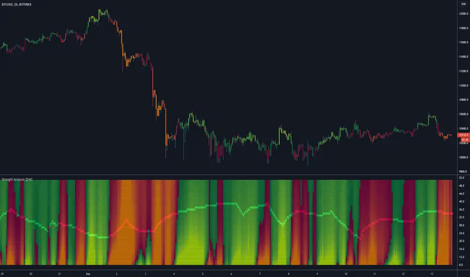
Strength Analyzer [DW]This is an experimental hybrid between relative strength and spectrum analysis methods aimed to deliver useful insights about cyclical dominance and momentum.
This study utilizes a modified RSI formula and a modified Goertzel algorithm to determine relative strength and spectral dominance for periods 8 through 50.
These periods are theorized by many analysts to be the main cyclical components of market movement.
In this study, you are given the option to apply equalization (EQ) to the dataset before estimating strength.
This enables you to transform your data and observe how strength estimates changes as well.
Whether you want to give emphasis to some frequencies, isolate specific bands, or completely alter the shape of your waveform, EQ filtration makes for an interesting experience.
The default EQ preset in this script cuts low end presence, dampens high frequency oscillations, and cleanly passes main cyclic components.
There are many ways to use EQ to transform your dataset, so play around with the settings and find the presets that work best for your analysis setup.
After EQ processing, the data is then passed through the modified RSI algorithm to generate momentum information
The modified RSI in this script is rescaled to oscillate between -1 and 1, and has the option to pass through a 2 pole Butterworth low pass filter before and after processing for a smoother output.
The strength thresholds are determined by the threshold value, which quantifies distance above and below 0.
The threshold value can also be thought of as conventional RSI distance from 50 rescaled so that an increment of 0.1 is equivalent to an increment of 5 on a conventional RSI.
A threshold value of 0.4 is equivalent to thresholds of 70 and 30 on a conventional RSI, so this is the default. The maximum threshold value is 1, which is equivalent to thresholds of 100 and 0.
This script plots colored sections for each period value using a gradient color scheme based on their respective strength estimates.
The color scheme in this script is a multicolored gradient that shows green scaled colors for bullish strength and red scaled colors for bearish strength.
Darker, less vibrant colors indicate lower strength. Brighter, more vibrant colors indicate higher strength.
Strength values near 0 will show the darkest colors, and values near the positive or negative threshold value will show the brightest.
The data is fed parallel through the modified Goertzel algorithm to obtain cyclic power information and to estimate the dominant cycle.
Gerald Goertzel's algorithm is a unique Fourier related transform that identifies tonal properties by quantifying resonance in a set of second order IIR filters with direct-form structure.
It is computationally more efficient than typical DFT or FFT algorithms, and yields decent spectral resolution.
In this variation of the algorithm, data is first passed through a 2 pole high pass filter to attenuate spectral dilation, then passed through a Hamming Window to tidy up the frequency range.
The clean windowed data is then passed through a recursive resonance loop over the frequency block to calculate filter coefficients, which are then used to identify real and imaginary magnitude components.
From there, the magnitude components are used to calculate cyclic power.
The power outputs of each period are then compared for dominant cycle estimation, which is plotted over the gradient.
The dominant cycle can also be optionally smoothed or halved based on your preferences.
Bar colors are included in this script. The color scheme is a gradient based on dominant cycle momentum.
Signals and alert conditions are included in this script as well, and can be customized to your liking.
The two main signal types in this script are:
-> Dominant Cycle - Signals based on dominant cycle or half dominant cycle changes from positive to negative strength or vice versa.
-> Confluence - Signals based on confluence emergence. Based on the majority of measured cycles or all measured cycles showing positive or negative strength.
The signals in this are also externally accessible by other scripts.
The output format is 1 for long signals, and -1 for short signals.
To integrate these signals with your own system, use a source input in your script and assign it to this script's "Direction Signals" output variable from the dropdown tab.
In addition, I included two external output variables that show dominant cycle strength and average cycle strength.
They can be integrated into your own scripts by using a source input and selecting the proper output variable, just like the signals.
The Strength Analyzer is a versatile and powerful analytical tool to have in the arsenal for generating unique insights about momentum and cycle dominance.
By analyzing strength on a spectral basis, we can look at relative price movements on a deeper level and gain insights that aren't necessarily obvious from simply looking at a price chart.
------------------------------------------------
This is a premium script, and access is provided on an invite-only basis.
To gain access, get a copy of the script overview, or for any other inquiries, send me a direct message!
I look forward to hearing from you!
------------------------------------------------
General Disclaimer:
Trading stocks, futures, Forex, options, ETFs, cryptocurrencies or any other financial instrument has large potential rewards, but also large potential risk.
You must be aware of the risks and be willing to accept them in order to invest in stocks, futures, Forex, options, ETFs or cryptocurrencies.
Don’t trade with money you can’t afford to lose.
This is neither a solicitation nor an offer to Buy/Sell stocks, futures, Forex, options, ETFs, cryptocurrencies or any other financial instrument.
No representation is being made that any account will or is likely to achieve profits or losses of any kind.
The past performance of any trading system or methodology is not necessarily indicative of future results.
------------------------------------------------
Note:
Because TV's UI can't handle displaying style options for 43 fills with 42 colors, the color scheme of the analyzer is currently not editable.
However, no other sacrifices to functionality or quality were made in this project.
As the TV team performs updates on the platform, the ability to customize this color scheme will likely come as well.
Also, it's important to note that this script uses a heavy amount of calculations to generate this output.
At times (very infrequently), TV will throw an error message saying "Calculation Takes Too Long", likely due to a momentary lull in available server space.
If you receive this error, simply hide then unhide the indicator, and everything should function as expected.
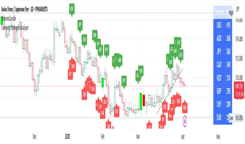
Currency Strength AnalyzerThis indicator calculates and ranks the strength of eight major currencies (AUD, CAD, CHF, EUR, GBP, JPY, NZD, USD) based on a stochastic-based scoring system. It retrieves forex pair data and determines each currency's relative strength using a customized scoring method.
Features:
Uses stochastic (Stoch) indicators to calculate bullish/bearish strength.
Aggregates scores for each currency based on multiple forex pairs.
Sorts currencies from strongest to weakest.
Displays results in a dynamically updated table.
Highlights the strongest and weakest currencies on the chart.
This tool helps traders identify potential trends and reversals in the forex market by visually comparing currency strengths in real-time.
Supertrend with RSI FilterThis indicator is an enhanced version of the classic Supertrend, incorporating an RSI (Relative Strength Index) filter to refine trend signals. Here is a detailed explanation of its functionality and key advantages over the traditional Supertrend.
1. Indicator Functionality
The indicator uses ATR (Average True Range) to calculate the Supertrend line, just like the classic version. However, it introduces an additional condition based on RSI to strengthen or weaken the Supertrend color based on market momentum.
2. Interpretation of Colors
The indicator displays the Supertrend line with dynamic colors based on trend direction and RSI strength:
- Uptrend (Supertrend in buy mode):
- Dark green (Teal): RSI above the defined threshold (default 50) → Strong bullish confirmation.
- Light gray: RSI below the threshold → Indicates a weaker uptrend or lack of confirmation.
- Downtrend (Supertrend in sell mode):
- Dark red: RSI below the threshold → Strong bearish confirmation.
- Light gray: RSI above the threshold → Indicates a weaker downtrend or lack of confirmation.
The opacity of the color dynamically adjusts based on how far RSI is from its threshold. The greater the difference, the more vivid the color, signaling a stronger trend.
3. Key Advantages Over the Classic Supertrend
- Filters out false signals: The RSI integration helps reduce false signals by only validating trends when RSI aligns with the Supertrend direction.
- Weakens uncertain signals: When RSI is close to its threshold, the color becomes more transparent, alerting traders to a less reliable trend.
- Classic mode available: The 'Use Classic Supertrend' option allows switching to a standard Supertrend display (fixed red/green) without the RSI effect.
4. Customizable Parameters
- ATR Length & ATR Factor: Define the sensitivity of the Supertrend.
- RSI Period & RSI Threshold: Allow refining the RSI filter based on market volatility.
- Classic mode: Enables/disables the RSI filtering to revert to the original Supertrend.
This indicator is especially valuable for traders looking to refine their trend signals based on market momentum measured by RSI.
This indicator is for informational purposes only and should not be considered financial advice. Trading involves risks, and past performance does not guarantee future results. Always conduct your own analysis before making any trading decisions.

AI x Meme Impulse Tracker [QuantraSystems]AI x Meme Impulse Tracker
Quantra Systems guarantees that the information created and published within this document and on the Tradingview platform is fully compliant with applicable regulations, does not constitute investment advice, and is not exclusively intended for qualified investors.
Important Note!
The system equity curve presented here has been generated as part of the process of testing and verifying the methodology behind this script.
Crucially, it was developed after the system was conceptualized, designed, and created, which helps to mitigate the risk of overfitting to historical data. In other words, the system was built for robustness, not for simply optimizing past performance.
This ensures that the system is less likely to degrade in performance over time, compared to hyper-optimized systems that are tailored to past data. No tweaks or optimizations were made to this system post-backtest.
Even More Important Note!!
The nature of markets is that they change quickly and unpredictably. Past performance does not guarantee future results - this is a fundamental rule in trading and investing.
While this system is designed with broad, flexible conditions to adapt quickly to a range of market environments, it is essential to understand that no assumptions should be made about future returns based on historical data. Markets are inherently uncertain, and this system - like all trading systems - cannot predict future outcomes.
Introduction
The AI x Meme Impulse Tracker is a cutting-edge, fast-acting rotational algorithm designed to capitalize on the strength of assets within pre-selected categories. Using a custom function built on top of the RSI Pulsar, the system measures momentum through impulses rather than traditional trend following methods. This allows for swifter reallocations based on short bursts of strength.
This system focuses on precision and agility - making it highly adaptable in volatile markets. The strategy is built around three independent asset categories - with allocations only made to the strongest asset in each - ensuring that capital movement (in particular between blockchains) is kept to a minimum for efficiency purposes while maintaining exposure to the highest performing tokens.
Legend
Token Inputs:
The Impulse Tracker is designed with dynamic asset selection - allowing traders to customize the inputs for each category. This feature enables flexible system management, as the number of active tokens within each category can be adjusted at any time. Whether the user chooses the default of 13 tokens per category, or fewer, the system will automatically recalibrate. This ensures that all calculations, from relative strength to individual performance assessments, adjust as required. Disabled tokens are treated by the system as if they don’t exist - seamlessly updating performance metrics and the Impulse Tracker’s allocation behavior to maintain the highest level of efficiency and accuracy.
System Equity Curve:
The Impulse Tracker plots both the rotational system’s equity and the Buy-and-Hold (or ‘HODL’) benchmark of Bitcoin for comparison. While the HODL approach allocates the entire portfolio to Bitcoin and functions as an index to compare to, the Impulse Tracker dynamically allocates based on strength impulses within the chosen tokens and categories. The system equity curve is representative of adding an equal capital split between the strongest assets of each category. The relative strength system does handle ‘ties’ of strength - in this situation multiple tokens from a single category can be included in the final equity curve, with the allocated weight to that category split between the tied assets.
TABLES:
Equity Stats:
This table is held in Quantra System's typical UI design language. It offers a comprehensive snapshot of the system’s performance, with key metrics organized to help traders quickly assess both short-term and cumulative results. The left side provides details on individual asset performance, while the right side presents a comparison of the system’s risk-adjusted metrics against a simple BTC Hodl strategy.
The leftmost column of the Equity Stats table showcases performance indicators for the system’s current allocations. This provides quick identification of the current strongest tokens, based on confirmed and non-repainting data as soon as the current opens and the last bar closes.
The right-hand side compares the performance differences between the system and Hodl profits, both on a cumulative basis and analyzing only the previous bar. The total number of position changes is also tracked in this table - an important metric when calculating total slippage and should be used to determine how ‘hands-on’ the strategy will be on the current timeframe.
The lower part of the table highlights a direct comparison of the AI x Memes Impulse strategy with buy-and-hold Bitcoin. The risk adjusted performance ratios, Sharpe, Sortino and Omega, are shown side by side, as well as the maximum drawdown experienced by both strategies within the set testing window.
Screener Table:
This table provides a detailed breakdown of the performance for each asset that has been the strongest in its category at some point and thus received an allocation. The table tracks several key metrics for each asset - including returns, volatility, Sharpe ratio, Sortino ratio, Omega ratio, and maximum drawdown. It also displays the signals for both current and previous periods, as well as the assets weight in the theoretical portfolio. Assets that have never received a signal are also included, giving traders an overview of which assets have contributed to the portfolio's performance and which have not played a role so far.
The position changes cell also offers important insights, as it shows the frequency of not just total position changes, but also rebalancing events.
Detailed Slippage Table:
The Detailed Slippage Table provides a comprehensive breakdown of the calculated slippage and fees incurred throughout the strategy’s operations. It contains several key metrics that give traders a granular view of the costs associated with executing the system:
Selected Slippage - Displays the current slippage rate, as defined in the input menu.
Removal Slippage - This accounts for any slippage or fees incurred when removing an allocation from a token.
Reallocation Slippage - Tracks the slippage or fees when reallocating capital to existing positions.
Addition Slippage - Measures the slippage or fees incurred when allocating capital to new tokens.
Final Slippage - Is the sum of all the individual slippage points and provides a quick view of the total slippage accounted for by the system.
The table is also divided into two columns:
Last Transaction Slippage + Fees - Displays any slippage or fees incurred based on position changes within the current bar.
Total Slippage + Fees - Shows the cumulative slippage and fees incurred since the portfolio’s selected start date.
Visual Customization:
Several customizable features are included within the input menu to enhance user experience. These include custom color palettes, both preloaded and user-selectable. This allows traders to personalize the visual appearance of the tables, ensuring clarity and consistency with their preferred interface themes and background coloring.
Additionally, users can adjust both the position and sizes of all the tables - enabling complete tailoring to the trader’s layout and specific viewing preferences and screen configurations. This level of customization ensures a more intuitive and flexible interaction with the system’s data.
Core Features and Methodologies
Advanced Risk Management - A Unique Filtering Approach:
The Equity Curve Activation Filter introduces an innovative way to dynamically manage capital allocation, aligning with periods of market trend strength. This filter is rooted in the understanding that markets move cyclically - altering between periods trending and mean-reverting periods. This cycle is especially pronounced in the crypto markets, where strong uptrends are often followed by prolonged periods of sideways movements or corrections as participants take profits and momentum fades.
The Cyclical Nature of Markets and Trend Following:
Financial markets do not trend indefinitely. Each uptrend or downtrend, whether over high and low timeframes, tends to culminate in a phase where momentum exhausts - leading to the sideways or corrective phases. This cycle results from the natural dynamics of market participants: during extended trends, more participants jump in, riding the momentum until profit taking causes the trend to slow down or reverse. This cyclical behavior occurs across all timeframes and in all markets - making it essential to adapt trading strategies in attempt to minimize losses during less favorable conditions.
In a trend following system, profitability often mirrors this cyclical pattern. Trend following strategies thrive when markets are moving directionally, capturing gains as price moves with strength in a single direction. However in phases where the market chops sideways, trend following strategies will usually experience drawdowns and reduced returns due to the impersistent nature of any trends. This fluctuation in trend following profitability can actually serve as one of the best coincident indicators of broader market regime change - when profitability begins to fade, it often signals a transition to drawn out unfavorable trend trading conditions.
The Equity Curve as a Market Signal
Within the Impulse Tracker, a continuous equity curve is calculated based upon the system's allocation to the strongest tokens. This equity curve effectively tracks the system’s performance under all market conditions. However, instead of solely relying on the direct performance of the selected tokens, the system applies additional filters to analyze the trend strength of this equity curve itself.
In the same way you only want to purchase an asset that is moving up in price, you only want to allocate capital to a strategy whose equity curve is trending upwards!
The Equity Curve Activation Filter consistently monitors the trend of this equity curve through various filter indicators, such as the “Wave Pendulum Trend”, the “Quasar QSM” and the “MAQSM” (an aggregate of multiple types of averages). These filters help determine whether the equity curve is trending upwards, signaling a favorable period for trend following. When the equity curve is in a positive trend, capital is allocated to the system as normal - allowing it to capture gains during favorable market conditions, Conversely, when the trend weakens and the equity curves begins to stagnate or decline, the activation filter shifts the system into a “cash” positions - temporarily halting allocations in order to prevent market exposure during choppy or mean reverting phases.
Timing Allocation With Market Conditions
This unique filtering approach ensures that the system is primarily active during periods when market trends are most supportive. By aligning capital allocations with the uptrend in trend following profitability, the system is designed to enter during periods of strong momentum and move to cash when momentum with the equity curve wanes. This approach reduces the risk of overtrading in less favorable conditions and preserves capital for the next favorable trend.
In essence the Equity Curve Allocation Filter serves as a dynamic risk management layer that leverages the cyclicality of trend following profitability in order to navigate shifting market phases.
Sensitivity and Signal Responsiveness:
The Quasar Sensitivity Setting allows users to fine-tune the system’s responsiveness to asset signals. High sensitivity settings lead to quicker position changes, making the system highly reactive to short term strength impulses. This is especially useful in fast moving markets where token strength can shift rapidly. The Sensitive setting might be more applicable to higher volatility or lower market cap assets - as the increased volatility increases the necessity of faster position cutting in order to front run the crowd. Of course - a balanced approach is ideal, as if the signals are too fast there will be too many whips and false signals. (And extra fees + slippage!)
The benefit of this script is because of the advanced slippage calculations, false signals are sufficiently punished (unlike systems without fees or slippage) - so it will become immediately apparent if the false signals have a significantly detrimental impact on the system’s equity curve.
Asset specific signals within each category are re-evaluated after the close of each bar to ensure that capital is always allocated to the highest performing asset. If a token’s momentum begins to fade the system swiftly reallocates to the next strongest asset within that category.
Category Filter - Allocates only to the Strongest Asset per group
One of the core innovations of the AI x Meme Impulse Tracker is the customizable Category Filter, which ensures that only the strongest-performing asset within each predefined group receives capital allocation. This approach not only increases the precision of asset selection but also allows traders to tailor the system to specific token narratives or categories. Sectors can include trending themes such as high-attention meme tokens, AI-driven tokens, or even categorize assets by blockchain ecosystems like Ethereum, Solana, or Base chain. This flexibility enables users to align their strategies with the latest market narratives or to optimize for specific groups, focusing on high-beta tokens within well defined sectors for a more targeted exposure. By keeping the focus on category leaders, the system avoids diluting its impact across underperforming assets, thereby maximizing capital efficiency and reducing unnecessary trading costs.
Dynamic Asset Reallocation:
Dynamic reallocation ensures that the system remains nimble and adapts to changing market conditions. Unlike slower systems, the Quasar method continually monitors for changes in asset strength and reallocates capital accordingly - ensuring that the system is always positioned in the highest performing assets within each category.
Position Changes and Slippage:
The Impulse Tracker places a strong emphasis on realistic simulation, prioritizing accuracy over inflated backtest results. This approach ensures that slippage is accounted for in a more aggressive manner than what may be experienced in real-world execution.
Each position change within the system - whether it’s buying, selling, reallocating, or rebalancing between assets - incurs slippage. Slippage is applied to both ends of every transaction: when a position is entered and exited, and when reallocating capital from one token to another. This dynamic behavior is further enhanced by a customizable slippage/fees input, allowing users to simulate realistic transaction costs based on their own market conditions and execution behaviors.
The slippage model works by applying a weighted slippage to the equity curve, taking into account the actual amount of capital being moved. Slippage is not applied in a blanket manner but rather in proportion to the allocation changes. For example, if the system reallocates from a single 100% position to two 50% allocations, slippage will be applied to the 50% removed from the first asset and the 50% added to the new asset, resulting in a 1x slippage multiplier.
This process becomes more granular when multiple assets are involved. For instance, if reallocating from two 50% positions to three 33% positions, slippage will be incurred on each of the changes, but at a reduced rate (⅔ x slippage), reflecting the smaller percentage of portfolio equity being moved. The slippage model accounts for all types of allocation shifts, whether increasing or decreasing the number of tokens held, providing a realistic assessment of system costs.
Here are some detailed examples to illustrate how slippage is calculated based on different scenarios:
100% → 50% / 50%: 1x slippage applied to both position changes (2 allocation changes).
50% / 50% → 33% / 33% / 33%: ⅔ x slippage multiplier applied across 3 allocation changes.
33% / 33% / 33% → 100%: 4/3 x slippage multiplier applied across 3 allocation changes.
In practice, not every position change will be rebalanced perfectly, leading to a lower number of transactions and lower costs in practice. Additionally, with the use of limit orders, a trader can easily reduce the costs of entering a position, as well as ensuring a competitive entry price.
By simulating slippage in this granular manner, the system captures the absolute maximum level of fees and slippage, in order to ensure that backtest results lean towards an underrepresentation - opposed to inflated results compared with practical execution.
A Special Note on Slippage
In the image above, the system has been applied to four different timeframes - 20h, 15h, 10h, and 5h - using identical settings and a selected slippage amount of 2%. By isolating a recent trend leg, we can illustrate an important concept: while the 15h timeframe is more profitable than the 20h timeframe, this difference stems from a core trading principle. Lower timeframes typically provide more data points and allow for quicker entries and exits in a robust system. This often results in reduced downside and compounding of gains.
However, slippage, fees, and execution constraints are limiting factors, especially in volatile, low-cap cryptocurrencies. Although lower timeframes can improve performance by increasing trade frequency, each trade incurs heavy slippage costs that accumulate - impacting the portfolio’s capital at a compounding rate. In this example, the chosen slippage rate of 2% per trade is designed to reflect the realistic trading costs, emphasizing how lower timeframe trading comes at the cost of increased slippage and fees
Finding the optimal balance between timeframe and slippage impact requires careful consideration of factors such as portfolio size, liquidity of selected tokens, execution speed, and the fee rate of the exchange you execute trades on.
Equity Curve and Performance Calculations
To provide a benchmark, the script also generates a Buy-and-Hold (or "HODL") equity curve that represents a complete allocation to Bitcoin. This allows users to easily compare the performance of the dynamic rotation system with that more traditional benchmark strategy.
The script tracks key performance metrics for both the dynamic portfolio and the HODL strategy, including:
Sharpe Ratio
The Sharpe Ratio is a key metric that evaluates a portfolio’s risk-adjusted return by comparing its ‘excess’ return to its volatility. Traditionally, the Sharpe Ratio measures returns relative to a risk-free rate. However, in our system’s calculation, we omit the risk-free rate and instead measure returns above a benchmark of 0%. This adjustment provides a more universal comparison, especially in the context of highly volatile assets like cryptocurrencies, where a traditional risk-free benchmark, such as the usual 3-month T-bills, is often irrelevant or too distant from the realities of the crypto market.
By using 0% as the baseline, we focus purely on the strategy's ability to generate raw returns in the face of market risk, which makes it easier to compare performance across different strategies or asset classes. In an environment like cryptocurrency, where volatility can be extreme, the importance of relative return against a highly volatile backdrop outweighs comparisons to a risk-free rate that bears little resemblance to the risk profile of digital assets.
Sortino Ratio
The Sortino Ratio improves upon the Sharpe Ratio by specifically targeting downside risk and leaves the upside potential untouched. In contrast to the Sharpe Ratio (which penalizes both upside and downside volatility), the Sortino Ratio focuses only on negative return deviations. This makes it a more suitable metric for evaluating strategies like the AI x Meme Impulse Tracker - that aim to minimize drawdowns without restricting upside capture. By measuring returns relative to a 0% baseline, the Sortino ratio provides a clearer assessment of how well the system generates gains while avoiding substantial losses in highly volatile markets like crypto.
Omega Ratio
The Omega Ratio is calculated as the ratio of gains to losses across all return thresholds, providing a more complete view of how the system balances upside and downside risk even compared to the Sortino Ratio. While it achieves a similar outcome to the Sortino Ratio by emphasizing the system's ability to capture gains while limiting losses, it is technically a mathematically superior method. However, we include both the Omega and Sortino ratios in our metric table, as the Sortino Ratio remains more widely recognized and commonly understood by traders and investors of all levels.
Usage Summary:
While the backtests in this description are generated as if a trader held a portfolio of just the strongest tokens, this was mainly designed as a method of logical verification and not a recommended investment strategy. In practice, this system can be used in multiple ways.
It can be used as above, or as a factor in forming part of a broader asset selection system, or even a method of filtering tokens by strength in order to inform a day trader which tokens might be optimal to look for long-only trading setups on an intrabar timeframe.
Final Summary:
The AI x Meme Impulse Tracker is a powerful algorithm that leverages a unique strength and impulse based approach to asset allocation within high beta token categories. Built with a robust risk management framework, the system’s Equity Curve Activation Filter dynamically manages capital exposure based on the cyclical nature of market trends, minimizing exposure during weaker phases.
With highly customizable settings, the Impulse Tracker enables precise capital allocation to only the strongest assets, informed by real-time metrics and rigorous slippage modeling in order to provide the best view of historical profitability. This adaptable design, coupled with advanced performance analytics, makes it a versatile tool for traders seeking an edge in fast moving and volatile crypto markets.
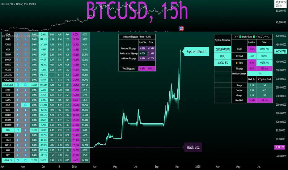
GKD-B Multi-Ticker Stepped Baseline [Loxx]Giga Kaleidoscope GKD-B Multi-Ticker Stepped Baseline is a Baseline module included in Loxx's "Giga Kaleidoscope Modularized Trading System".
This version of the GKD-B Baseline is designed specifically to support traders who wish to conduct GKD-BT Multi-Ticker Backtests with multiple tickers. This functionality is exclusive to the GKD-BT Multi-Ticker Backtests.
Traders have the capability to apply a filter to the selected moving average, leveraging various volatility metrics to enhance trend identification. This feature is tailored for traders favoring a gradual and consistent approach, enabling them to discern more sustainable trends. The system permits filtering for both the input data and the moving average results, requiring price movements to exceed a specific threshold—defined as multiples of the volatility—before acknowledging a trend change. This mechanism effectively reduces false signals caused by market noise and lateral movements. A distinctive aspect of this tool is its ability to adjust both price and moving average data based on volatility indicators like VIX, EUVIX, BVIV, and EVIV, among others. Understanding the time frame over which a volatility index is measured is crucial; for instance, VIX is measured on an annual basis, whereas BVIV and EVIV are based on a 30-day period. To accurately convert these measurements to a daily scale, users must input the correct "days per year" value: 252 for VIX and 30 for BVIV and EVIV. Future updates will introduce additional functionality to extend analysis across various time frames, but currently, this feature is solely available for daily time frame analysis.
█ GKD-B Multi-Ticker Stepped Baseline includes 65+ different moving averages:
Adaptive Moving Average - AMA
ADXvma - Average Directional Volatility Moving Average
Ahrens Moving Average
Alexander Moving Average - ALXMA
Deviation Scaled Moving Average - DSMA
Donchian
Double Exponential Moving Average - DEMA
Double Smoothed Exponential Moving Average - DSEMA
Double Smoothed FEMA - DSFEMA
Double Smoothed Range Weighted EMA - DSRWEMA
Double Smoothed Wilders EMA - DSWEMA
Double Weighted Moving Average - DWMA
Ehlers Optimal Tracking Filter - EOTF
Exponential Moving Average - EMA
Fast Exponential Moving Average - FEMA
Fractal Adaptive Moving Average - FRAMA
Generalized DEMA - GDEMA
Generalized Double DEMA - GDDEMA
Hull Moving Average (Type 1) - HMA1
Hull Moving Average (Type 2) - HMA2
Hull Moving Average (Type 3) - HMA3
Hull Moving Average (Type 4) - HMA4
IE /2 - Early T3 by Tim Tilson
Integral of Linear Regression Slope - ILRS
Kaufman Adaptive Moving Average - KAMA
Laguerre Filter
Leader Exponential Moving Average
Linear Regression Value - LSMA ( Least Squares Moving Average )
Linear Weighted Moving Average - LWMA
McGinley Dynamic
McNicholl EMA
Non-Lag Moving Average
Ocean NMA Moving Average - ONMAMA
One More Moving Average - OMA
Parabolic Weighted Moving Average
Probability Density Function Moving Average - PDFMA
Quadratic Regression Moving Average - QRMA
Regularized EMA - REMA
Range Weighted EMA - RWEMA
Recursive Moving Trendline
Simple Decycler - SDEC
Simple Jurik Moving Average - SJMA
Simple Moving Average - SMA
Sine Weighted Moving Average
Smoothed LWMA - SLWMA
Smoothed Moving Average - SMMA
Smoother
Super Smoother
T3
Three-pole Ehlers Butterworth
Three-pole Ehlers Smoother
Triangular Moving Average - TMA
Triple Exponential Moving Average - TEMA
Two-pole Ehlers Butterworth
Two-pole Ehlers smoother
Variable Index Dynamic Average - VIDYA
Variable Moving Average - VMA
Volume Weighted EMA - VEMA
Volume Weighted Moving Average - VWMA
Zero-Lag DEMA - Zero Lag Exponential Moving Average
Zero-Lag Moving Average
Zero Lag TEMA - Zero Lag Triple Exponential Moving Average
Geometric Mean Moving Average
Coral
Tether Lines
Range Filter
Triangle Moving Average Generalized
Ultinate Smoother
Adaptive Moving Average - AMA
The Adaptive Moving Average (AMA) is a moving average that changes its sensitivity to price moves depending on the calculated volatility. It becomes more sensitive during periods when the price is moving smoothly in a certain direction and becomes less sensitive when the price is volatile.
ADXvma - Average Directional Volatility Moving Average
Linnsoft's ADXvma formula is a volatility-based moving average, with the volatility being determined by the value of the ADX indicator.
The ADXvma has the SMA in Chande's CMO replaced with an EMA , it then uses a few more layers of EMA smoothing before the "Volatility Index" is calculated.
A side effect is, those additional layers slow down the ADXvma when you compare it to Chande's Variable Index Dynamic Average VIDYA .
The ADXVMA provides support during uptrends and resistance during downtrends and will stay flat for longer, but will create some of the most accurate market signals when it decides to move.
Ahrens Moving Average
Richard D. Ahrens's Moving Average promises "Smoother Data" that isn't influenced by the occasional price spike. It works by using the Open and the Close in his formula so that the only time the Ahrens Moving Average will change is when the candlestick is either making new highs or new lows.
Alexander Moving Average - ALXMA
This Moving Average uses an elaborate smoothing formula and utilizes a 7 period Moving Average. It corresponds to fitting a second-order polynomial to seven consecutive observations. This moving average is rarely used in trading but is interesting as this Moving Average has been applied to diffusion indexes that tend to be very volatile.
Deviation Scaled Moving Average - DSMA
The Deviation-Scaled Moving Average is a data smoothing technique that acts like an exponential moving average with a dynamic smoothing coefficient. The smoothing coefficient is automatically updated based on the magnitude of price changes. In the Deviation-Scaled Moving Average, the standard deviation from the mean is chosen to be the measure of this magnitude. The resulting indicator provides substantial smoothing of the data even when price changes are small while quickly adapting to these changes.
Donchian
Donchian Channels are three lines generated by moving average calculations that comprise an indicator formed by upper and lower bands around a midrange or median band. The upper band marks the highest price of a security over N periods while the lower band marks the lowest price of a security over N periods.
Double Exponential Moving Average - DEMA
The Double Exponential Moving Average ( DEMA ) combines a smoothed EMA and a single EMA to provide a low-lag indicator. It's primary purpose is to reduce the amount of "lagging entry" opportunities, and like all Moving Averages, the DEMA confirms uptrends whenever price crosses on top of it and closes above it, and confirms downtrends when the price crosses under it and closes below it - but with significantly less lag.
Double Smoothed Exponential Moving Average - DSEMA
The Double Smoothed Exponential Moving Average is a lot less laggy compared to a traditional EMA . It's also considered a leading indicator compared to the EMA , and is best utilized whenever smoothness and speed of reaction to market changes are required.
Double Smoothed FEMA - DSFEMA
Same as the Double Exponential Moving Average (DEMA), but uses a faster version of EMA for its calculation.
Double Smoothed Range Weighted EMA - DSRWEMA
Range weighted exponential moving average (EMA) is, unlike the "regular" range weighted average calculated in a different way. Even though the basis - the range weighting - is the same, the way how it is calculated is completely different. By definition this type of EMA is calculated as a ratio of EMA of price*weight / EMA of weight. And the results are very different and the two should be considered as completely different types of averages. The higher than EMA to price changes responsiveness when the ranges increase remains in this EMA too and in those cases this EMA is clearly leading the "regular" EMA. This version includes double smoothing.
Double Smoothed Wilders EMA - DSWEMA
Welles Wilder was frequently using one "special" case of EMA (Exponential Moving Average) that is due to that fact (that he used it) sometimes called Wilder's EMA. This version is adding double smoothing to Wilder's EMA in order to make it "faster" (it is more responsive to market prices than the original) and is still keeping very smooth values.
Double Weighted Moving Average - DWMA
Double weighted moving average is an LWMA (Linear Weighted Moving Average). Instead of doing one cycle for calculating the LWMA, the indicator is made to cycle the loop 2 times. That produces a smoother values than the original LWMA
Ehlers Optimal Tracking Filter - EOTF
The Elher's Optimum Tracking Filter quickly adjusts rapid shifts in the price and yet is relatively smooth when the price has a sideways action. The operation of this filter is similar to Kaufman’s Adaptive Moving
Average
Exponential Moving Average - EMA
The EMA places more significance on recent data points and moves closer to price than the SMA ( Simple Moving Average ). It reacts faster to volatility due to its emphasis on recent data and is known for its ability to give greater weight to recent and more relevant data. The EMA is therefore seen as an enhancement over the SMA .
Fast Exponential Moving Average - FEMA
An Exponential Moving Average with a short look-back period.
Fractal Adaptive Moving Average - FRAMA
The Fractal Adaptive Moving Average by John Ehlers is an intelligent adaptive Moving Average which takes the importance of price changes into account and follows price closely enough to display significant moves whilst remaining flat if price ranges. The FRAMA does this by dynamically adjusting the look-back period based on the market's fractal geometry.
Generalized DEMA - GDEMA
The double exponential moving average (DEMA), was developed by Patrick Mulloy in an attempt to reduce the amount of lag time found in traditional moving averages. It was first introduced in the February 1994 issue of the magazine Technical Analysis of Stocks & Commodities in Mulloy's article "Smoothing Data with Faster Moving Averages.". Instead of using fixed multiplication factor in the final DEMA formula, the generalized version allows you to change it. By varying the "volume factor" form 0 to 1 you apply different multiplications and thus producing DEMA with different "speed" - the higher the volume factor is the "faster" the DEMA will be (but also the slope of it will be less smooth). The volume factor is limited in the calculation to 1 since any volume factor that is larger than 1 is increasing the overshooting to the extent that some volume factors usage makes the indicator unusable.
Generalized Double DEMA - GDDEMA
The double exponential moving average (DEMA), was developed by Patrick Mulloy in an attempt to reduce the amount of lag time found in traditional moving averages. It was first introduced in the February 1994 issue of the magazine Technical Analysis of Stocks & Commodities in Mulloy's article "Smoothing Data with Faster Moving Averages''. This is an extension of the Generalized DEMA using Tim Tillsons (the inventor of T3) idea, and is using GDEMA of GDEMA for calculation (which is the "middle step" of T3 calculation). Since there are no versions showing that middle step, this version covers that too. The result is smoother than Generalized DEMA, but is less smooth than T3 - one has to do some experimenting in order to find the optimal way to use it, but in any case, since it is "faster" than the T3 (Tim Tillson T3) and still smooth, it looks like a good compromise between speed and smoothness.
Hull Moving Average (Type 1) - HMA1
Alan Hull's HMA makes use of weighted moving averages to prioritize recent values and greatly reduce lag whilst maintaining the smoothness of a traditional Moving Average. For this reason, it's seen as a well-suited Moving Average for identifying entry points. This version uses SMA for smoothing.
Hull Moving Average (Type 2) - HMA2
Alan Hull's HMA makes use of weighted moving averages to prioritize recent values and greatly reduce lag whilst maintaining the smoothness of a traditional Moving Average. For this reason, it's seen as a well-suited Moving Average for identifying entry points. This version uses EMA for smoothing.
Hull Moving Average (Type 3) - HMA3
Alan Hull's HMA makes use of weighted moving averages to prioritize recent values and greatly reduce lag whilst maintaining the smoothness of a traditional Moving Average. For this reason, it's seen as a well-suited Moving Average for identifying entry points. This version uses LWMA for smoothing.
Hull Moving Average (Type 4) - HMA4
Alan Hull's HMA makes use of weighted moving averages to prioritize recent values and greatly reduce lag whilst maintaining the smoothness of a traditional Moving Average. For this reason, it's seen as a well-suited Moving Average for identifying entry points. This version uses SMMA for smoothing.
IE /2 - Early T3 by Tim Tilson and T3 new
The T3 moving average is a type of technical indicator used in financial analysis to identify trends in price movements. It is similar to the Exponential Moving Average (EMA) and the Double Exponential Moving Average (DEMA), but uses a different smoothing algorithm.
The T3 moving average is calculated using a series of exponential moving averages that are designed to filter out noise and smooth the data. The resulting smoothed data is then weighted with a non-linear function to produce a final output that is more responsive to changes in trend direction.
The T3 moving average can be customized by adjusting the length of the moving average, as well as the weighting function used to smooth the data. It is commonly used in conjunction with other technical indicators as part of a larger trading strategy.
Integral of Linear Regression Slope - ILRS
A Moving Average where the slope of a linear regression line is simply integrated as it is fitted in a moving window of length N (natural numbers in maths) across the data. The derivative of ILRS is the linear regression slope. ILRS is not the same as a SMA ( Simple Moving Average ) of length N, which is actually the midpoint of the linear regression line as it moves across the data.
Kaufman Adaptive Moving Average - KAMA
Developed by Perry Kaufman, Kaufman's Adaptive Moving Average (KAMA) is a moving average designed to account for market noise or volatility. KAMA will closely follow prices when the price swings are relatively small and the noise is low.
Laguerre Filter
The Laguerre Filter is a smoothing filter which is based on Laguerre polynomials. The filter requires the current price, three prior prices, a user defined factor called Alpha to fill its calculation.
Adjusting the Alpha coefficient is used to increase or decrease its lag and its smoothness.
Leader Exponential Moving Average
The Leader EMA was created by Giorgos E. Siligardos who created a Moving Average which was able to eliminate lag altogether whilst maintaining some smoothness. It was first described during his research paper "MACD Leader" where he applied this to the MACD to improve its signals and remove its lagging issue. This filter uses his leading MACD's "modified EMA" and can be used as a zero lag filter.
Linear Regression Value - LSMA ( Least Squares Moving Average )
LSMA as a Moving Average is based on plotting the end point of the linear regression line. It compares the current value to the prior value and a determination is made of a possible trend, eg. the linear regression line is pointing up or down.
Linear Weighted Moving Average - LWMA
LWMA reacts to price quicker than the SMA and EMA . Although it's similar to the Simple Moving Average , the difference is that a weight coefficient is multiplied to the price which means the most recent price has the highest weighting, and each prior price has progressively less weight. The weights drop in a linear fashion.
McGinley Dynamic
John McGinley created this Moving Average to track prices better than traditional Moving Averages. It does this by incorporating an automatic adjustment factor into its formula, which speeds (or slows) the indicator in trending, or ranging, markets.
McNicholl EMA
Dennis McNicholl developed this Moving Average to use as his center line for his "Better Bollinger Bands" indicator and was successful because it responded better to volatility changes over the standard SMA and managed to avoid common whipsaws.
Non-lag moving average
The Non Lag Moving average follows price closely and gives very quick signals as well as early signals of price change. As a standalone Moving Average, it should not be used on its own, but as an additional confluence tool for early signals.
Ocean NMA Moving Average - ONMAMA
Created by Jim Sloman, the NMA is a moving average that automatically adjusts to volatility without being programmed to do so. For more info, read his guide "Ocean Theory, an Introduction"
One More Moving Average (OMA)
The One More Moving Average (OMA) is a technical indicator that calculates a series of Jurik-style moving averages in order to reduce noise and provide smoother price data. It uses six exponential moving averages to generate the final value, with the length of the moving averages determined by an adaptive algorithm that adjusts to the current market conditions. The algorithm calculates the average period by comparing the signal to noise ratio and using this value to determine the length of the moving averages. The resulting values are used to generate the final value of the OMA, which can be used to identify trends and potential changes in trend direction.
Parabolic Weighted Moving Average
The Parabolic Weighted Moving Average is a variation of the Linear Weighted Moving Average . The Linear Weighted Moving Average calculates the average by assigning different weights to each element in its calculation. The Parabolic Weighted Moving Average is a variation that allows weights to be changed to form a parabolic curve. It is done simply by using the Power parameter of this indicator.
Probability Density Function Moving Average - PDFMA
Probability density function based MA is a sort of weighted moving average that uses probability density function to calculate the weights. By its nature it is similar to a lot of digital filters.
Quadratic Regression Moving Average - QRMA
A quadratic regression is the process of finding the equation of the parabola that best fits a set of data. This moving average is an obscure concept that was posted to Forex forums in around 2008.
Regularized EMA - REMA
The regularized exponential moving average (REMA) by Chris Satchwell is a variation on the EMA (see Exponential Moving Average) designed to be smoother but not introduce too much extra lag.
Range Weighted EMA - RWEMA
This indicator is a variation of the range weighted EMA. The variation comes from a possible need to make that indicator a bit less "noisy" when it comes to slope changes. The method used for calculating this variation is the method described by Lee Leibfarth in his article "Trading With An Adaptive Price Zone".
Recursive Moving Trendline
Dennis Meyers's Recursive Moving Trendline uses a recursive (repeated application of a rule) polynomial fit, a technique that uses a small number of past values estimations of price and today's price to predict tomorrow's price.
Simple Decycler - SDEC
The Ehlers Simple Decycler study is a virtually zero-lag technical indicator proposed by John F. Ehlers. The original idea behind this study (and several others created by John F. Ehlers) is that market data can be considered a continuum of cycle periods with different cycle amplitudes. Thus, trending periods can be considered segments of longer cycles, or, in other words, low-frequency segments. Applying the right filter might help identify these segments.
Simple Loxx Moving Average - SLMA
A three stage moving average combining an adaptive EMA, a Kalman Filter, and a Kauffman adaptive filter.
Simple Moving Average - SMA
The SMA calculates the average of a range of prices by adding recent prices and then dividing that figure by the number of time periods in the calculation average. It is the most basic Moving Average which is seen as a reliable tool for starting off with Moving Average studies. As reliable as it may be, the basic moving average will work better when it's enhanced into an EMA .
Sine Weighted Moving Average
The Sine Weighted Moving Average assigns the most weight at the middle of the data set. It does this by weighting from the first half of a Sine Wave Cycle and the most weighting is given to the data in the middle of that data set. The Sine WMA closely resembles the TMA (Triangular Moving Average).
Smoothed LWMA - SLWMA
A smoothed version of the LWMA
Smoothed Moving Average - SMMA
The Smoothed Moving Average is similar to the Simple Moving Average ( SMA ), but aims to reduce noise rather than reduce lag. SMMA takes all prices into account and uses a long lookback period. Due to this, it's seen as an accurate yet laggy Moving Average.
Smoother
The Smoother filter is a faster-reacting smoothing technique which generates considerably less lag than the SMMA ( Smoothed Moving Average ). It gives earlier signals but can also create false signals due to its earlier reactions. This filter is sometimes wrongly mistaken for the superior Jurik Smoothing algorithm.
Super Smoother
The Super Smoother filter uses John Ehlers’s “Super Smoother” which consists of a Two pole Butterworth filter combined with a 2-bar SMA ( Simple Moving Average ) that suppresses the 22050 Hz Nyquist frequency: A characteristic of a sampler, which converts a continuous function or signal into a discrete sequence.
Three-pole Ehlers Butterworth
The 3 pole Ehlers Butterworth (as well as the Two pole Butterworth) are both superior alternatives to the EMA and SMA . They aim at producing less lag whilst maintaining accuracy. The 2 pole filter will give you a better approximation for price, whereas the 3 pole filter has superior smoothing.
Three-pole Ehlers smoother
The 3 pole Ehlers smoother works almost as close to price as the above mentioned 3 Pole Ehlers Butterworth. It acts as a strong baseline for signals but removes some noise. Side by side, it hardly differs from the Three Pole Ehlers Butterworth but when examined closely, it has better overshoot reduction compared to the 3 pole Ehlers Butterworth.
Triangular Moving Average - TMA
The TMA is similar to the EMA but uses a different weighting scheme. Exponential and weighted Moving Averages will assign weight to the most recent price data. Simple moving averages will assign the weight equally across all the price data. With a TMA (Triangular Moving Average), it is double smoother (averaged twice) so the majority of the weight is assigned to the middle portion of the data.
Triple Exponential Moving Average - TEMA
The TEMA uses multiple EMA calculations as well as subtracting lag to create a tool which can be used for scalping pullbacks. As it follows price closely, its signals are considered very noisy and should only be used in extremely fast-paced trading conditions.
Two-pole Ehlers Butterworth
The 2 pole Ehlers Butterworth (as well as the three pole Butterworth mentioned above) is another filter that cuts out the noise and follows the price closely. The 2 pole is seen as a faster, leading filter over the 3 pole and follows price a bit more closely. Analysts will utilize both a 2 pole and a 3 pole Butterworth on the same chart using the same period, but having both on chart allows its crosses to be traded.
Two-pole Ehlers smoother
A smoother version of the Two pole Ehlers Butterworth. This filter is the faster version out of the 3 pole Ehlers Butterworth. It does a decent job at cutting out market noise whilst emphasizing a closer following to price over the 3 pole Ehlers .
Variable Index Dynamic Average - VIDYA
Variable Index Dynamic Average Technical Indicator ( VIDYA ) was developed by Tushar Chande. It is an original method of calculating the Exponential Moving Average ( EMA ) with the dynamically changing period of averaging.
Variable Moving Average - VMA
The Variable Moving Average (VMA) is a study that uses an Exponential Moving Average being able to automatically adjust its smoothing factor according to the market volatility.
Volume Weighted EMA - VEMA
An EMA that uses a volume and price weighted calculation instead of the standard price input.
Volume Weighted Moving Average - VWMA
A Volume Weighted Moving Average is a moving average where more weight is given to bars with heavy volume than with light volume. Thus the value of the moving average will be closer to where most trading actually happened than it otherwise would be without being volume weighted.
Zero-Lag DEMA - Zero Lag Double Exponential Moving Average
John Ehlers's Zero Lag DEMA's aim is to eliminate the inherent lag associated with all trend following indicators which average a price over time. Because this is a Double Exponential Moving Average with Zero Lag, it has a tendency to overshoot and create a lot of false signals for swing trading. It can however be used for quick scalping or as a secondary indicator for confluence.
Zero-Lag Moving Average
The Zero Lag Moving Average is described by its creator, John Ehlers , as a Moving Average with absolutely no delay. And it's for this reason that this filter will cause a lot of abrupt signals which will not be ideal for medium to long-term traders. This filter is designed to follow price as close as possible whilst de-lagging data instead of basing it on regular data. The way this is done is by attempting to remove the cumulative effect of the Moving Average.
Zero-Lag TEMA - Zero Lag Triple Exponential Moving Average
Just like the Zero Lag DEMA , this filter will give you the fastest signals out of all the Zero Lag Moving Averages. This is useful for scalping but dangerous for medium to long-term traders, especially during market Volatility and news events. Having no lag, this filter also has no smoothing in its signals and can cause some very bizarre behavior when applied to certain indicators.
█ Volatility Goldie Locks Zone
This volatility filter is the standard first pass filter that is used for all NNFX systems despite the additional volatility/volume filter used in step 5. For this filter, price must fall into a range of maximum and minimum values calculated using multiples of volatility. Unlike the standard NNFX systems, this version of volatility filtering is separated from the core Baseline and uses it's own moving average with Loxx's Exotic Source Types.
█ Volatility Types included
The GKD system utilizes volatility-based take profits and stop losses. Each take profit and stop loss is calculated as a multiple of volatility. You can change the values of the multipliers in the settings as well.
This module includes 17 types of volatility:
Close-to-Close
Parkinson
Garman-Klass
Rogers-Satchell
Yang-Zhang
Garman-Klass-Yang-Zhang
Exponential Weighted Moving Average
Standard Deviation of Log Returns
Pseudo GARCH(2,2)
Average True Range
True Range Double
Standard Deviation
Adaptive Deviation
Median Absolute Deviation
Efficiency-Ratio Adaptive ATR
Mean Absolute Deviation
Static Percent
Various volatility estimators and indicators that investors and traders can use to measure the dispersion or volatility of a financial instrument's price. Each estimator has its strengths and weaknesses, and the choice of estimator should depend on the specific needs and circumstances of the user.
Volatility Ticker Selection
Import volatility tickers like VIX, EUVIX, BVIV, and EVIV.
Close-to-Close
Close-to-Close volatility is a classic and widely used volatility measure, sometimes referred to as historical volatility.
Volatility is an indicator of the speed of a stock price change. A stock with high volatility is one where the price changes rapidly and with a larger amplitude. The more volatile a stock is, the riskier it is.
Close-to-close historical volatility is calculated using only a stock's closing prices. It is the simplest volatility estimator. However, in many cases, it is not precise enough. Stock prices could jump significantly during a trading session and return to the opening value at the end. That means that a considerable amount of price information is not taken into account by close-to-close volatility.
Despite its drawbacks, Close-to-Close volatility is still useful in cases where the instrument doesn't have intraday prices. For example, mutual funds calculate their net asset values daily or weekly, and thus their prices are not suitable for more sophisticated volatility estimators.
Parkinson
Parkinson volatility is a volatility measure that uses the stock’s high and low price of the day.
The main difference between regular volatility and Parkinson volatility is that the latter uses high and low prices for a day, rather than only the closing price. This is useful as close-to-close prices could show little difference while large price movements could have occurred during the day. Thus, Parkinson's volatility is considered more precise and requires less data for calculation than close-to-close volatility.
One drawback of this estimator is that it doesn't take into account price movements after the market closes. Hence, it systematically undervalues volatility. This drawback is addressed in the Garman-Klass volatility estimator.
Garman-Klass
Garman-Klass is a volatility estimator that incorporates open, low, high, and close prices of a security.
Garman-Klass volatility extends Parkinson's volatility by taking into account the opening and closing prices. As markets are most active during the opening and closing of a trading session, it makes volatility estimation more accurate.
Garman and Klass also assumed that the process of price change follows a continuous diffusion process (Geometric Brownian motion). However, this assumption has several drawbacks. The method is not robust for opening jumps in price and trend movements.
Despite its drawbacks, the Garman-Klass estimator is still more effective than the basic formula since it takes into account not only the price at the beginning and end of the time interval but also intraday price extremes.
Researchers Rogers and Satchell have proposed a more efficient method for assessing historical volatility that takes into account price trends. See Rogers-Satchell Volatility for more detail.
Rogers-Satchell
Rogers-Satchell is an estimator for measuring the volatility of securities with an average return not equal to zero.
Unlike Parkinson and Garman-Klass estimators, Rogers-Satchell incorporates a drift term (mean return not equal to zero). As a result, it provides better volatility estimation when the underlying is trending.
The main disadvantage of this method is that it does not take into account price movements between trading sessions. This leads to an underestimation of volatility since price jumps periodically occur in the market precisely at the moments between sessions.
A more comprehensive estimator that also considers the gaps between sessions was developed based on the Rogers-Satchel formula in the 2000s by Yang-Zhang. See Yang Zhang Volatility for more detail.
Yang-Zhang
Yang Zhang is a historical volatility estimator that handles both opening jumps and the drift and has a minimum estimation error.
Yang-Zhang volatility can be thought of as a combination of the overnight (close-to-open volatility) and a weighted average of the Rogers-Satchell volatility and the day’s open-to-close volatility. It is considered to be 14 times more efficient than the close-to-close estimator.
Garman-Klass-Yang-Zhang
Garman-Klass-Yang-Zhang (GKYZ) volatility estimator incorporates the returns of open, high, low, and closing prices in its calculation.
GKYZ volatility estimator takes into account overnight jumps but not the trend, i.e., it assumes that the underlying asset follows a Geometric Brownian Motion (GBM) process with zero drift. Therefore, the GKYZ volatility estimator tends to overestimate the volatility when the drift is different from zero. However, for a GBM process, this estimator is eight times more efficient than the close-to-close volatility estimator.
Exponential Weighted Moving Average
The Exponentially Weighted Moving Average (EWMA) is a quantitative or statistical measure used to model or describe a time series. The EWMA is widely used in finance, with the main applications being technical analysis and volatility modeling.
The moving average is designed such that older observations are given lower weights. The weights decrease exponentially as the data point gets older – hence the name exponentially weighted.
The only decision a user of the EWMA must make is the parameter lambda. The parameter decides how important the current observation is in the calculation of the EWMA. The higher the value of lambda, the more closely the EWMA tracks the original time series.
Standard Deviation of Log Returns
This is the simplest calculation of volatility. It's the standard deviation of ln(close/close(1)).
Pseudo GARCH(2,2)
This is calculated using a short- and long-run mean of variance multiplied by ?.
avg(var;M) + (1 ? ?) avg(var;N) = 2?var/(M+1-(M-1)L) + 2(1-?)var/(M+1-(M-1)L)
Solving for ? can be done by minimizing the mean squared error of estimation; that is, regressing L^-1var - avg(var; N) against avg(var; M) - avg(var; N) and using the resulting beta estimate as ?.
Average True Range
The average true range (ATR) is a technical analysis indicator, introduced by market technician J. Welles Wilder Jr. in his book New Concepts in Technical Trading Systems, that measures market volatility by decomposing the entire range of an asset price for that period.
The true range indicator is taken as the greatest of the following: current high less the current low; the absolute value of the current high less the previous close; and the absolute value of the current low less the previous close. The ATR is then a moving average, generally using 14 days, of the true ranges.
True Range Double
A special case of ATR that attempts to correct for volatility skew.
Standard Deviation
Standard deviation is a statistic that measures the dispersion of a dataset relative to its mean and is calculated as the square root of the variance. The standard deviation is calculated as the square root of variance by determining each data point's deviation relative to the mean. If the data points are further from the mean, there is a higher deviation within the data set; thus, the more spread out the data, the higher the standard deviation.
Adaptive Deviation
By definition, the Standard Deviation (STD, also represented by the Greek letter sigma ? or the Latin letter s) is a measure that is used to quantify the amount of variation or dispersion of a set of data values. In technical analysis, we usually use it to measure the level of current volatility.
Standard Deviation is based on Simple Moving Average calculation for mean value. This version of standard deviation uses the properties of EMA to calculate what can be called a new type of deviation, and since it is based on EMA, we can call it EMA deviation. Additionally, Perry Kaufman's efficiency ratio is used to make it adaptive (since all EMA type calculations are nearly perfect for adapting).
The difference when compared to the standard is significant--not just because of EMA usage, but the efficiency ratio makes it a "bit more logical" in very volatile market conditions.
Median Absolute Deviation
The median absolute deviation is a measure of statistical dispersion. Moreover, the MAD is a robust statistic, being more resilient to outliers in a data set than the standard deviation. In the standard deviation, the distances from the mean are squared, so large deviations are weighted more heavily, and thus outliers can heavily influence it. In the MAD, the deviations of a small number of outliers are irrelevant.
Because the MAD is a more robust estimator of scale than the sample variance or standard deviation, it works better with distributions without a mean or variance, such as the Cauchy distribution.
For this indicator, a manual recreation of the quantile function in Pine Script is used. This is so users have a full inside view into how this is calculated.
Efficiency-Ratio Adaptive ATR
Average True Range (ATR) is a widely used indicator for many occasions in technical analysis. It is calculated as the RMA of the true range. This version adds a "twist": it uses Perry Kaufman's Efficiency Ratio to calculate adaptive true range.
Mean Absolute Deviation
The mean absolute deviation (MAD) is a measure of variability that indicates the average distance between observations and their mean. MAD uses the original units of the data, which simplifies interpretation. Larger values signify that the data points spread out further from the average. Conversely, lower values correspond to data points bunching closer to it. The mean absolute deviation is also known as the mean deviation and average absolute deviation.
This definition of the mean absolute deviation sounds similar to the standard deviation (SD). While both measure variability, they have different calculations. In recent years, some proponents of MAD have suggested that it replace the SD as the primary measure because it is a simpler concept that better fits real life.
█ Giga Kaleidoscope Modularized Trading System
Core components of an NNFX algorithmic trading strategy
The NNFX algorithm is built on the principles of trend, momentum, and volatility. There are six core components in the NNFX trading algorithm:
1. Volatility - price volatility; e.g., Average True Range, True Range Double, Close-to-Close, etc.
2. Baseline - a moving average to identify price trend
3. Confirmation 1 - a technical indicator used to identify trends
4. Confirmation 2 - a technical indicator used to identify trends
5. Continuation - a technical indicator used to identify trends
6. Volatility/Volume - a technical indicator used to identify volatility/volume breakouts/breakdown
7. Exit - a technical indicator used to determine when a trend is exhausted
8. Metamorphosis - a technical indicator that produces a compound signal from the combination of other GKD indicators*
*(not part of the NNFX algorithm)
What is Volatility in the NNFX trading system?
In the NNFX (No Nonsense Forex) trading system, ATR (Average True Range) is typically used to measure the volatility of an asset. It is used as a part of the system to help determine the appropriate stop loss and take profit levels for a trade. ATR is calculated by taking the average of the true range values over a specified period.
True range is calculated as the maximum of the following values:
-Current high minus the current low
-Absolute value of the current high minus the previous close
-Absolute value of the current low minus the previous close
ATR is a dynamic indicator that changes with changes in volatility. As volatility increases, the value of ATR increases, and as volatility decreases, the value of ATR decreases. By using ATR in NNFX system, traders can adjust their stop loss and take profit levels according to the volatility of the asset being traded. This helps to ensure that the trade is given enough room to move, while also minimizing potential losses.
Other types of volatility include True Range Double (TRD), Close-to-Close, and Garman-Klass
What is a Baseline indicator?
The baseline is essentially a moving average, and is used to determine the overall direction of the market.
The baseline in the NNFX system is used to filter out trades that are not in line with the long-term trend of the market. The baseline is plotted on the chart along with other indicators, such as the Moving Average (MA), the Relative Strength Index (RSI), and the Average True Range (ATR).
Trades are only taken when the price is in the same direction as the baseline. For example, if the baseline is sloping upwards, only long trades are taken, and if the baseline is sloping downwards, only short trades are taken. This approach helps to ensure that trades are in line with the overall trend of the market, and reduces the risk of entering trades that are likely to fail.
By using a baseline in the NNFX system, traders can have a clear reference point for determining the overall trend of the market, and can make more informed trading decisions. The baseline helps to filter out noise and false signals, and ensures that trades are taken in the direction of the long-term trend.
What is a Confirmation indicator?
Confirmation indicators are technical indicators that are used to confirm the signals generated by primary indicators. Primary indicators are the core indicators used in the NNFX system, such as the Average True Range (ATR), the Moving Average (MA), and the Relative Strength Index (RSI).
The purpose of the confirmation indicators is to reduce false signals and improve the accuracy of the trading system. They are designed to confirm the signals generated by the primary indicators by providing additional information about the strength and direction of the trend.
Some examples of confirmation indicators that may be used in the NNFX system include the Bollinger Bands, the MACD (Moving Average Convergence Divergence), and the MACD Oscillator. These indicators can provide information about the volatility, momentum, and trend strength of the market, and can be used to confirm the signals generated by the primary indicators.
In the NNFX system, confirmation indicators are used in combination with primary indicators and other filters to create a trading system that is robust and reliable. By using multiple indicators to confirm trading signals, the system aims to reduce the risk of false signals and improve the overall profitability of the trades.
What is a Continuation indicator?
In the NNFX (No Nonsense Forex) trading system, a continuation indicator is a technical indicator that is used to confirm a current trend and predict that the trend is likely to continue in the same direction. A continuation indicator is typically used in conjunction with other indicators in the system, such as a baseline indicator, to provide a comprehensive trading strategy.
What is a Volatility/Volume indicator?
Volume indicators, such as the On Balance Volume (OBV), the Chaikin Money Flow (CMF), or the Volume Price Trend (VPT), are used to measure the amount of buying and selling activity in a market. They are based on the trading volume of the market, and can provide information about the strength of the trend. In the NNFX system, volume indicators are used to confirm trading signals generated by the Moving Average and the Relative Strength Index. Volatility indicators include Average Direction Index, Waddah Attar, and Volatility Ratio. In the NNFX trading system, volatility is a proxy for volume and vice versa.
By using volume indicators as confirmation tools, the NNFX trading system aims to reduce the risk of false signals and improve the overall profitability of trades. These indicators can provide additional information about the market that is not captured by the primary indicators, and can help traders to make more informed trading decisions. In addition, volume indicators can be used to identify potential changes in market trends and to confirm the strength of price movements.
What is an Exit indicator?
The exit indicator is used in conjunction with other indicators in the system, such as the Moving Average (MA), the Relative Strength Index (RSI), and the Average True Range (ATR), to provide a comprehensive trading strategy.
The exit indicator in the NNFX system can be any technical indicator that is deemed effective at identifying optimal exit points. Examples of exit indicators that are commonly used include the Parabolic SAR, and the Average Directional Index (ADX).
The purpose of the exit indicator is to identify when a trend is likely to reverse or when the market conditions have changed, signaling the need to exit a trade. By using an exit indicator, traders can manage their risk and prevent significant losses.
In the NNFX system, the exit indicator is used in conjunction with a stop loss and a take profit order to maximize profits and minimize losses. The stop loss order is used to limit the amount of loss that can be incurred if the trade goes against the trader, while the take profit order is used to lock in profits when the trade is moving in the trader's favor.
Overall, the use of an exit indicator in the NNFX trading system is an important component of a comprehensive trading strategy. It allows traders to manage their risk effectively and improve the profitability of their trades by exiting at the right time.
What is an Metamorphosis indicator?
The concept of a metamorphosis indicator involves the integration of two or more GKD indicators to generate a compound signal. This is achieved by evaluating the accuracy of each indicator and selecting the signal from the indicator with the highest accuracy. As an illustration, let's consider a scenario where we calculate the accuracy of 10 indicators and choose the signal from the indicator that demonstrates the highest accuracy.
The resulting output from the metamorphosis indicator can then be utilized in a GKD-BT backtest by occupying a slot that aligns with the purpose of the metamorphosis indicator. The slot can be a GKD-B, GKD-C, or GKD-E slot, depending on the specific requirements and objectives of the indicator. This allows for seamless integration and utilization of the compound signal within the GKD-BT framework.
How does Loxx's GKD (Giga Kaleidoscope Modularized Trading System) implement the NNFX algorithm outlined above?
Loxx's GKD v2.0 system has five types of modules (indicators/strategies). These modules are:
1. GKD-BT - Backtesting module (Volatility, Number 1 in the NNFX algorithm)
2. GKD-B - Baseline module (Baseline and Volatility/Volume, Numbers 1 and 2 in the NNFX algorithm)
3. GKD-C - Confirmation 1/2 and Continuation module (Confirmation 1/2 and Continuation, Numbers 3, 4, and 5 in the NNFX algorithm)
4. GKD-V - Volatility/Volume module (Confirmation 1/2, Number 6 in the NNFX algorithm)
5. GKD-E - Exit module (Exit, Number 7 in the NNFX algorithm)
6. GKD-M - Metamorphosis module (Metamorphosis, Number 8 in the NNFX algorithm, but not part of the NNFX algorithm)
(additional module types will added in future releases)
Each module interacts with every module by passing data to A backtest module wherein the various components of the GKD system are combined to create a trading signal.
That is, the Baseline indicator passes its data to Volatility/Volume. The Volatility/Volume indicator passes its values to the Confirmation 1 indicator. The Confirmation 1 indicator passes its values to the Confirmation 2 indicator. The Confirmation 2 indicator passes its values to the Continuation indicator. The Continuation indicator passes its values to the Exit indicator, and finally, the Exit indicator passes its values to the Backtest strategy.
This chaining of indicators requires that each module conform to Loxx's GKD protocol, therefore allowing for the testing of every possible combination of technical indicators that make up the six components of the NNFX algorithm.
What does the application of the GKD trading system look like?
Example trading system:
Backtest: Multi-Ticker CC Backtest
Baseline: Hull Moving Average
Volatility/Volume: Hurst Exponent
Confirmation 1: Advance Trend Pressure as shown on the chart above
Confirmation 2: uf2018
Continuation: Coppock Curve
Exit: Rex Oscillator
Metamorphosis: Baseline Optimizer
Each GKD indicator is denoted with a module identifier of either: GKD-BT, GKD-B, GKD-C, GKD-V, GKD-M, or GKD-E. This allows traders to understand to which module each indicator belongs and where each indicator fits into the GKD system.
█ Giga Kaleidoscope Modularized Trading System Signals
Standard Entry
1. GKD-C Confirmation gives signal
2. Baseline agrees
3. Price inside Goldie Locks Zone Minimum
4. Price inside Goldie Locks Zone Maximum
5. Confirmation 2 agrees
6. Volatility/Volume agrees
1-Candle Standard Entry
1a. GKD-C Confirmation gives signal
2a. Baseline agrees
3a. Price inside Goldie Locks Zone Minimum
4a. Price inside Goldie Locks Zone Maximum
Next Candle
1b. Price retraced
2b. Baseline agrees
3b. Confirmation 1 agrees
4b. Confirmation 2 agrees
5b. Volatility/Volume agrees
Baseline Entry
1. GKD-B Baseline gives signal
2. Confirmation 1 agrees
3. Price inside Goldie Locks Zone Minimum
4. Price inside Goldie Locks Zone Maximum
5. Confirmation 2 agrees
6. Volatility/Volume agrees
7. Confirmation 1 signal was less than 'Maximum Allowable PSBC Bars Back' prior
1-Candle Baseline Entry
1a. GKD-B Baseline gives signal
2a. Confirmation 1 agrees
3a. Price inside Goldie Locks Zone Minimum
4a. Price inside Goldie Locks Zone Maximum
5a. Confirmation 1 signal was less than 'Maximum Allowable PSBC Bars Back' prior
Next Candle
1b. Price retraced
2b. Baseline agrees
3b. Confirmation 1 agrees
4b. Confirmation 2 agrees
5b. Volatility/Volume agrees
Volatility/Volume Entry
1. GKD-V Volatility/Volume gives signal
2. Confirmation 1 agrees
3. Price inside Goldie Locks Zone Minimum
4. Price inside Goldie Locks Zone Maximum
5. Confirmation 2 agrees
6. Baseline agrees
7. Confirmation 1 signal was less than 7 candles prior
1-Candle Volatility/Volume Entry
1a. GKD-V Volatility/Volume gives signal
2a. Confirmation 1 agrees
3a. Price inside Goldie Locks Zone Minimum
4a. Price inside Goldie Locks Zone Maximum
5a. Confirmation 1 signal was less than 'Maximum Allowable PSVVC Bars Back' prior
Next Candle
1b. Price retraced
2b. Volatility/Volume agrees
3b. Confirmation 1 agrees
4b. Confirmation 2 agrees
5b. Baseline agrees
Confirmation 2 Entry
1. GKD-C Confirmation 2 gives signal
2. Confirmation 1 agrees
3. Price inside Goldie Locks Zone Minimum
4. Price inside Goldie Locks Zone Maximum
5. Volatility/Volume agrees
6. Baseline agrees
7. Confirmation 1 signal was less than 7 candles prior
1-Candle Confirmation 2 Entry
1a. GKD-C Confirmation 2 gives signal
2a. Confirmation 1 agrees
3a. Price inside Goldie Locks Zone Minimum
4a. Price inside Goldie Locks Zone Maximum
5a. Confirmation 1 signal was less than 'Maximum Allowable PSC2C Bars Back' prior
Next Candle
1b. Price retraced
2b. Confirmation 2 agrees
3b. Confirmation 1 agrees
4b. Volatility/Volume agrees
5b. Baseline agrees
PullBack Entry
1a. GKD-B Baseline gives signal
2a. Confirmation 1 agrees
3a. Price is beyond 1.0x Volatility of Baseline
Next Candle
1b. Price inside Goldie Locks Zone Minimum
2b. Price inside Goldie Locks Zone Maximum
3b. Confirmation 1 agrees
4b. Confirmation 2 agrees
5b. Volatility/Volume agrees
Continuation Entry
1. Standard Entry, 1-Candle Standard Entry, Baseline Entry, 1-Candle Baseline Entry, Volatility/Volume Entry, 1-Candle Volatility/Volume Entry, Confirmation 2 Entry, 1-Candle Confirmation 2 Entry, or Pullback entry triggered previously
2. Baseline hasn't crossed since entry signal trigger
4. Confirmation 1 agrees
5. Baseline agrees
6. Confirmation 2 agrees

Machine Learning Momentum Index (MLMI) [Zeiierman]█ Overview
The Machine Learning Momentum Index (MLMI) represents the next step in oscillator trading. By blending traditional momentum analysis with machine learning, MLMI delivers a potent and dynamic tool that aligns with the complexities of modern financial landscapes. Offering traders an adaptive way to understand and act on market momentum and trends, this oscillator provides real-time insights into market momentum and prevailing trends.
█ How It Works:
Momentum Analysis: MLMI employs a dual-layer analysis, utilizing quick and slow weighted moving averages (WMA) of the Relative Strength Index (RSI) to gauge the market's momentum and direction.
Machine Learning Integration: Through the k-Nearest Neighbors (k-NN) algorithm, MLMI intelligently examines historical data to make more accurate momentum predictions, adapting to the intricate patterns of the market.
MLMI's precise calculation involves:
Weighted Moving Averages: Calculations of quick (5-period) and slow (20-period) WMAs of the RSI to track short-term and long-term momentum.
k-Nearest Neighbors Algorithm: Distances between current parameters and previous data are measured, and the nearest neighbors are used for predictive modeling.
Trend Analysis: Recognition of prevailing trends through the relationship between quick and slow-moving averages.
█ How to use
The Machine Learning Momentum Index (MLMI) can be utilized in much the same way as traditional trend and momentum oscillators, providing key insights into market direction and strength. What sets MLMI apart is its integration of artificial intelligence, allowing it to adapt dynamically to market changes and offer a more nuanced and responsive analysis.
Identifying Trend Direction and Strength: The MLMI serves as a tool to recognize market trends, signaling whether the momentum is upward or downward. It also provides insights into the intensity of the momentum, helping traders understand both the direction and strength of prevailing market trends.
Identifying Consolidation Areas: When the MLMI Prediction line and the WMA of the MLMI Prediction line become flat/oscillate around the mid-level, it's a strong sign that the market is in a consolidation phase. This insight from the MLMI allows traders to recognize periods of market indecision.
Recognizing Overbought or Oversold Conditions: By identifying levels where the market may be overbought or oversold, MLMI offers insights into potential price corrections or reversals.
█ Settings
Prediction Data (k)
This parameter controls the number of neighbors to consider while making a prediction using the k-Nearest Neighbors (k-NN) algorithm. By modifying the value of k, you can change how sensitive the prediction is to local fluctuations in the data.
A smaller value of k will make the prediction more sensitive to local variations and can lead to a more erratic prediction line.
A larger value of k will consider more neighbors, thus making the prediction more stable but potentially less responsive to sudden changes.
Trend length
This parameter controls the length of the trend used in computing the momentum. This length refers to the number of periods over which the momentum is calculated, affecting how quickly the indicator reacts to changes in the underlying price movements.
A shorter trend length (smaller momentumWindow) will make the indicator more responsive to short-term price changes, potentially generating more signals but at the risk of more false alarms.
A longer trend length (larger momentumWindow) will make the indicator smoother and less responsive to short-term noise, but it may lag in reacting to significant price changes.
Please note that the Machine Learning Momentum Index (MLMI) might not be effective on higher timeframes, such as daily or above. This limitation arises because there may not be enough data at these timeframes to provide accurate momentum and trend analysis. To overcome this challenge and make the most of what MLMI has to offer, it's recommended to use the indicator on lower timeframes.
-----------------
Disclaimer
The information contained in my Scripts/Indicators/Ideas/Algos/Systems does not constitute financial advice or a solicitation to buy or sell any securities of any type. I will not accept liability for any loss or damage, including without limitation any loss of profit, which may arise directly or indirectly from the use of or reliance on such information.
All investments involve risk, and the past performance of a security, industry, sector, market, financial product, trading strategy, backtest, or individual's trading does not guarantee future results or returns. Investors are fully responsible for any investment decisions they make. Such decisions should be based solely on an evaluation of their financial circumstances, investment objectives, risk tolerance, and liquidity needs.
My Scripts/Indicators/Ideas/Algos/Systems are only for educational purposes!

GKD-B Multi-Ticker Baseline [Loxx]Giga Kaleidoscope GKD-B Multi-Ticker Baseline is a Baseline module included in Loxx's "Giga Kaleidoscope Modularized Trading System".
This is a special implementation of GKD-B Baseline that allows the trader to input multiple tickers to be passed onto a GKD-BT Multi-Ticker Backtest. This baseline can only be used with the GKD-BT Multi-Ticker Backtests.
GKD-B Multi-Ticker Baseline includes 64 different moving averages:
Adaptive Moving Average - AMA
ADXvma - Average Directional Volatility Moving Average
Ahrens Moving Average
Alexander Moving Average - ALXMA
Deviation Scaled Moving Average - DSMA
Donchian
Double Exponential Moving Average - DEMA
Double Smoothed Exponential Moving Average - DSEMA
Double Smoothed FEMA - DSFEMA
Double Smoothed Range Weighted EMA - DSRWEMA
Double Smoothed Wilders EMA - DSWEMA
Double Weighted Moving Average - DWMA
Ehlers Optimal Tracking Filter - EOTF
Exponential Moving Average - EMA
Fast Exponential Moving Average - FEMA
Fractal Adaptive Moving Average - FRAMA
Generalized DEMA - GDEMA
Generalized Double DEMA - GDDEMA
Hull Moving Average (Type 1) - HMA1
Hull Moving Average (Type 2) - HMA2
Hull Moving Average (Type 3) - HMA3
Hull Moving Average (Type 4) - HMA4
IE /2 - Early T3 by Tim Tilson
Integral of Linear Regression Slope - ILRS
Instantaneous Trendline
Kalman Filter
Kaufman Adaptive Moving Average - KAMA
Laguerre Filter
Leader Exponential Moving Average
Linear Regression Value - LSMA ( Least Squares Moving Average )
Linear Weighted Moving Average - LWMA
McGinley Dynamic
McNicholl EMA
Non-Lag Moving Average
Ocean NMA Moving Average - ONMAMA
One More Moving Average - OMA
Parabolic Weighted Moving Average
Probability Density Function Moving Average - PDFMA
Quadratic Regression Moving Average - QRMA
Regularized EMA - REMA
Range Weighted EMA - RWEMA
Recursive Moving Trendline
Simple Decycler - SDEC
Simple Jurik Moving Average - SJMA
Simple Moving Average - SMA
Sine Weighted Moving Average
Smoothed LWMA - SLWMA
Smoothed Moving Average - SMMA
Smoother
Super Smoother
T3
Three-pole Ehlers Butterworth
Three-pole Ehlers Smoother
Triangular Moving Average - TMA
Triple Exponential Moving Average - TEMA
Two-pole Ehlers Butterworth
Two-pole Ehlers smoother
Variable Index Dynamic Average - VIDYA
Variable Moving Average - VMA
Volume Weighted EMA - VEMA
Volume Weighted Moving Average - VWMA
Zero-Lag DEMA - Zero Lag Exponential Moving Average
Zero-Lag Moving Average
Zero Lag TEMA - Zero Lag Triple Exponential Moving Average
Adaptive Moving Average - AMA
The Adaptive Moving Average (AMA) is a moving average that changes its sensitivity to price moves depending on the calculated volatility. It becomes more sensitive during periods when the price is moving smoothly in a certain direction and becomes less sensitive when the price is volatile.
ADXvma - Average Directional Volatility Moving Average
Linnsoft's ADXvma formula is a volatility-based moving average, with the volatility being determined by the value of the ADX indicator.
The ADXvma has the SMA in Chande's CMO replaced with an EMA , it then uses a few more layers of EMA smoothing before the "Volatility Index" is calculated.
A side effect is, those additional layers slow down the ADXvma when you compare it to Chande's Variable Index Dynamic Average VIDYA .
The ADXVMA provides support during uptrends and resistance during downtrends and will stay flat for longer, but will create some of the most accurate market signals when it decides to move.
Ahrens Moving Average
Richard D. Ahrens's Moving Average promises "Smoother Data" that isn't influenced by the occasional price spike. It works by using the Open and the Close in his formula so that the only time the Ahrens Moving Average will change is when the candlestick is either making new highs or new lows.
Alexander Moving Average - ALXMA
This Moving Average uses an elaborate smoothing formula and utilizes a 7 period Moving Average. It corresponds to fitting a second-order polynomial to seven consecutive observations. This moving average is rarely used in trading but is interesting as this Moving Average has been applied to diffusion indexes that tend to be very volatile.
Deviation Scaled Moving Average - DSMA
The Deviation-Scaled Moving Average is a data smoothing technique that acts like an exponential moving average with a dynamic smoothing coefficient. The smoothing coefficient is automatically updated based on the magnitude of price changes. In the Deviation-Scaled Moving Average, the standard deviation from the mean is chosen to be the measure of this magnitude. The resulting indicator provides substantial smoothing of the data even when price changes are small while quickly adapting to these changes.
Donchian
Donchian Channels are three lines generated by moving average calculations that comprise an indicator formed by upper and lower bands around a midrange or median band. The upper band marks the highest price of a security over N periods while the lower band marks the lowest price of a security over N periods.
Double Exponential Moving Average - DEMA
The Double Exponential Moving Average ( DEMA ) combines a smoothed EMA and a single EMA to provide a low-lag indicator. It's primary purpose is to reduce the amount of "lagging entry" opportunities, and like all Moving Averages, the DEMA confirms uptrends whenever price crosses on top of it and closes above it, and confirms downtrends when the price crosses under it and closes below it - but with significantly less lag.
Double Smoothed Exponential Moving Average - DSEMA
The Double Smoothed Exponential Moving Average is a lot less laggy compared to a traditional EMA . It's also considered a leading indicator compared to the EMA , and is best utilized whenever smoothness and speed of reaction to market changes are required.
Double Smoothed FEMA - DSFEMA
Same as the Double Exponential Moving Average (DEMA), but uses a faster version of EMA for its calculation.
Double Smoothed Range Weighted EMA - DSRWEMA
Range weighted exponential moving average (EMA) is, unlike the "regular" range weighted average calculated in a different way. Even though the basis - the range weighting - is the same, the way how it is calculated is completely different. By definition this type of EMA is calculated as a ratio of EMA of price*weight / EMA of weight. And the results are very different and the two should be considered as completely different types of averages. The higher than EMA to price changes responsiveness when the ranges increase remains in this EMA too and in those cases this EMA is clearly leading the "regular" EMA. This version includes double smoothing.
Double Smoothed Wilders EMA - DSWEMA
Welles Wilder was frequently using one "special" case of EMA (Exponential Moving Average) that is due to that fact (that he used it) sometimes called Wilder's EMA. This version is adding double smoothing to Wilder's EMA in order to make it "faster" (it is more responsive to market prices than the original) and is still keeping very smooth values.
Double Weighted Moving Average - DWMA
Double weighted moving average is an LWMA (Linear Weighted Moving Average). Instead of doing one cycle for calculating the LWMA, the indicator is made to cycle the loop 2 times. That produces a smoother values than the original LWMA
Ehlers Optimal Tracking Filter - EOTF
The Elher's Optimum Tracking Filter quickly adjusts rapid shifts in the price and yet is relatively smooth when the price has a sideways action. The operation of this filter is similar to Kaufman’s Adaptive Moving
Average
Exponential Moving Average - EMA
The EMA places more significance on recent data points and moves closer to price than the SMA ( Simple Moving Average ). It reacts faster to volatility due to its emphasis on recent data and is known for its ability to give greater weight to recent and more relevant data. The EMA is therefore seen as an enhancement over the SMA .
Fast Exponential Moving Average - FEMA
An Exponential Moving Average with a short look-back period.
Fractal Adaptive Moving Average - FRAMA
The Fractal Adaptive Moving Average by John Ehlers is an intelligent adaptive Moving Average which takes the importance of price changes into account and follows price closely enough to display significant moves whilst remaining flat if price ranges. The FRAMA does this by dynamically adjusting the look-back period based on the market's fractal geometry.
Generalized DEMA - GDEMA
The double exponential moving average (DEMA), was developed by Patrick Mulloy in an attempt to reduce the amount of lag time found in traditional moving averages. It was first introduced in the February 1994 issue of the magazine Technical Analysis of Stocks & Commodities in Mulloy's article "Smoothing Data with Faster Moving Averages.". Instead of using fixed multiplication factor in the final DEMA formula, the generalized version allows you to change it. By varying the "volume factor" form 0 to 1 you apply different multiplications and thus producing DEMA with different "speed" - the higher the volume factor is the "faster" the DEMA will be (but also the slope of it will be less smooth). The volume factor is limited in the calculation to 1 since any volume factor that is larger than 1 is increasing the overshooting to the extent that some volume factors usage makes the indicator unusable.
Generalized Double DEMA - GDDEMA
The double exponential moving average (DEMA), was developed by Patrick Mulloy in an attempt to reduce the amount of lag time found in traditional moving averages. It was first introduced in the February 1994 issue of the magazine Technical Analysis of Stocks & Commodities in Mulloy's article "Smoothing Data with Faster Moving Averages''. This is an extension of the Generalized DEMA using Tim Tillsons (the inventor of T3) idea, and is using GDEMA of GDEMA for calculation (which is the "middle step" of T3 calculation). Since there are no versions showing that middle step, this version covers that too. The result is smoother than Generalized DEMA, but is less smooth than T3 - one has to do some experimenting in order to find the optimal way to use it, but in any case, since it is "faster" than the T3 (Tim Tillson T3) and still smooth, it looks like a good compromise between speed and smoothness.
Hull Moving Average (Type 1) - HMA1
Alan Hull's HMA makes use of weighted moving averages to prioritize recent values and greatly reduce lag whilst maintaining the smoothness of a traditional Moving Average. For this reason, it's seen as a well-suited Moving Average for identifying entry points. This version uses SMA for smoothing.
Hull Moving Average (Type 2) - HMA2
Alan Hull's HMA makes use of weighted moving averages to prioritize recent values and greatly reduce lag whilst maintaining the smoothness of a traditional Moving Average. For this reason, it's seen as a well-suited Moving Average for identifying entry points. This version uses EMA for smoothing.
Hull Moving Average (Type 3) - HMA3
Alan Hull's HMA makes use of weighted moving averages to prioritize recent values and greatly reduce lag whilst maintaining the smoothness of a traditional Moving Average. For this reason, it's seen as a well-suited Moving Average for identifying entry points. This version uses LWMA for smoothing.
Hull Moving Average (Type 4) - HMA4
Alan Hull's HMA makes use of weighted moving averages to prioritize recent values and greatly reduce lag whilst maintaining the smoothness of a traditional Moving Average. For this reason, it's seen as a well-suited Moving Average for identifying entry points. This version uses SMMA for smoothing.
IE /2 - Early T3 by Tim Tilson and T3 new
The T3 moving average is a type of technical indicator used in financial analysis to identify trends in price movements. It is similar to the Exponential Moving Average (EMA) and the Double Exponential Moving Average (DEMA), but uses a different smoothing algorithm.
The T3 moving average is calculated using a series of exponential moving averages that are designed to filter out noise and smooth the data. The resulting smoothed data is then weighted with a non-linear function to produce a final output that is more responsive to changes in trend direction.
The T3 moving average can be customized by adjusting the length of the moving average, as well as the weighting function used to smooth the data. It is commonly used in conjunction with other technical indicators as part of a larger trading strategy.
Integral of Linear Regression Slope - ILRS
A Moving Average where the slope of a linear regression line is simply integrated as it is fitted in a moving window of length N (natural numbers in maths) across the data. The derivative of ILRS is the linear regression slope. ILRS is not the same as a SMA ( Simple Moving Average ) of length N, which is actually the midpoint of the linear regression line as it moves across the data.
Instantaneous Trendline
The Instantaneous Trendline is created by removing the dominant cycle component from the price information which makes this Moving Average suitable for medium to long-term trading.
Kalman Filter
Kalman filter is an algorithm that uses a series of measurements observed over time, containing statistical noise and other inaccuracies. This means that the filter was originally designed to work with noisy data. Also, it is able to work with incomplete data. Another advantage is that it is designed for and applied in dynamic systems; our price chart belongs to such systems. This version is true to the original design of the trade-ready Kalman Filter where velocity is the triggering mechanism.
Kalman Filter is a more accurate smoothing/prediction algorithm than the moving average because it is adaptive: it accounts for estimation errors and tries to adjust its predictions from the information it learned in the previous stage. Theoretically, Kalman Filter consists of measurement and transition components.
Kaufman Adaptive Moving Average - KAMA
Developed by Perry Kaufman, Kaufman's Adaptive Moving Average (KAMA) is a moving average designed to account for market noise or volatility. KAMA will closely follow prices when the price swings are relatively small and the noise is low.
Laguerre Filter
The Laguerre Filter is a smoothing filter which is based on Laguerre polynomials. The filter requires the current price, three prior prices, a user defined factor called Alpha to fill its calculation.
Adjusting the Alpha coefficient is used to increase or decrease its lag and its smoothness.
Leader Exponential Moving Average
The Leader EMA was created by Giorgos E. Siligardos who created a Moving Average which was able to eliminate lag altogether whilst maintaining some smoothness. It was first described during his research paper "MACD Leader" where he applied this to the MACD to improve its signals and remove its lagging issue. This filter uses his leading MACD's "modified EMA" and can be used as a zero lag filter.
Linear Regression Value - LSMA ( Least Squares Moving Average )
LSMA as a Moving Average is based on plotting the end point of the linear regression line. It compares the current value to the prior value and a determination is made of a possible trend, eg. the linear regression line is pointing up or down.
Linear Weighted Moving Average - LWMA
LWMA reacts to price quicker than the SMA and EMA . Although it's similar to the Simple Moving Average , the difference is that a weight coefficient is multiplied to the price which means the most recent price has the highest weighting, and each prior price has progressively less weight. The weights drop in a linear fashion.
McGinley Dynamic
John McGinley created this Moving Average to track prices better than traditional Moving Averages. It does this by incorporating an automatic adjustment factor into its formula, which speeds (or slows) the indicator in trending, or ranging, markets.
McNicholl EMA
Dennis McNicholl developed this Moving Average to use as his center line for his "Better Bollinger Bands" indicator and was successful because it responded better to volatility changes over the standard SMA and managed to avoid common whipsaws.
Non-lag moving average
The Non Lag Moving average follows price closely and gives very quick signals as well as early signals of price change. As a standalone Moving Average, it should not be used on its own, but as an additional confluence tool for early signals.
Ocean NMA Moving Average - ONMAMA
Created by Jim Sloman, the NMA is a moving average that automatically adjusts to volatility without being programmed to do so. For more info, read his guide "Ocean Theory, an Introduction"
One More Moving Average (OMA)
The One More Moving Average (OMA) is a technical indicator that calculates a series of Jurik-style moving averages in order to reduce noise and provide smoother price data. It uses six exponential moving averages to generate the final value, with the length of the moving averages determined by an adaptive algorithm that adjusts to the current market conditions. The algorithm calculates the average period by comparing the signal to noise ratio and using this value to determine the length of the moving averages. The resulting values are used to generate the final value of the OMA, which can be used to identify trends and potential changes in trend direction.
Parabolic Weighted Moving Average
The Parabolic Weighted Moving Average is a variation of the Linear Weighted Moving Average . The Linear Weighted Moving Average calculates the average by assigning different weights to each element in its calculation. The Parabolic Weighted Moving Average is a variation that allows weights to be changed to form a parabolic curve. It is done simply by using the Power parameter of this indicator.
Probability Density Function Moving Average - PDFMA
Probability density function based MA is a sort of weighted moving average that uses probability density function to calculate the weights. By its nature it is similar to a lot of digital filters.
Quadratic Regression Moving Average - QRMA
A quadratic regression is the process of finding the equation of the parabola that best fits a set of data. This moving average is an obscure concept that was posted to Forex forums in around 2008.
Regularized EMA - REMA
The regularized exponential moving average (REMA) by Chris Satchwell is a variation on the EMA (see Exponential Moving Average) designed to be smoother but not introduce too much extra lag.
Range Weighted EMA - RWEMA
This indicator is a variation of the range weighted EMA. The variation comes from a possible need to make that indicator a bit less "noisy" when it comes to slope changes. The method used for calculating this variation is the method described by Lee Leibfarth in his article "Trading With An Adaptive Price Zone".
Recursive Moving Trendline
Dennis Meyers's Recursive Moving Trendline uses a recursive (repeated application of a rule) polynomial fit, a technique that uses a small number of past values estimations of price and today's price to predict tomorrow's price.
Simple Decycler - SDEC
The Ehlers Simple Decycler study is a virtually zero-lag technical indicator proposed by John F. Ehlers. The original idea behind this study (and several others created by John F. Ehlers) is that market data can be considered a continuum of cycle periods with different cycle amplitudes. Thus, trending periods can be considered segments of longer cycles, or, in other words, low-frequency segments. Applying the right filter might help identify these segments.
Simple Loxx Moving Average - SLMA
A three stage moving average combining an adaptive EMA, a Kalman Filter, and a Kauffman adaptive filter.
Simple Moving Average - SMA
The SMA calculates the average of a range of prices by adding recent prices and then dividing that figure by the number of time periods in the calculation average. It is the most basic Moving Average which is seen as a reliable tool for starting off with Moving Average studies. As reliable as it may be, the basic moving average will work better when it's enhanced into an EMA .
Sine Weighted Moving Average
The Sine Weighted Moving Average assigns the most weight at the middle of the data set. It does this by weighting from the first half of a Sine Wave Cycle and the most weighting is given to the data in the middle of that data set. The Sine WMA closely resembles the TMA (Triangular Moving Average).
Smoothed LWMA - SLWMA
A smoothed version of the LWMA
Smoothed Moving Average - SMMA
The Smoothed Moving Average is similar to the Simple Moving Average ( SMA ), but aims to reduce noise rather than reduce lag. SMMA takes all prices into account and uses a long lookback period. Due to this, it's seen as an accurate yet laggy Moving Average.
Smoother
The Smoother filter is a faster-reacting smoothing technique which generates considerably less lag than the SMMA ( Smoothed Moving Average ). It gives earlier signals but can also create false signals due to its earlier reactions. This filter is sometimes wrongly mistaken for the superior Jurik Smoothing algorithm.
Super Smoother
The Super Smoother filter uses John Ehlers’s “Super Smoother” which consists of a Two pole Butterworth filter combined with a 2-bar SMA ( Simple Moving Average ) that suppresses the 22050 Hz Nyquist frequency: A characteristic of a sampler, which converts a continuous function or signal into a discrete sequence.
Three-pole Ehlers Butterworth
The 3 pole Ehlers Butterworth (as well as the Two pole Butterworth) are both superior alternatives to the EMA and SMA . They aim at producing less lag whilst maintaining accuracy. The 2 pole filter will give you a better approximation for price, whereas the 3 pole filter has superior smoothing.
Three-pole Ehlers smoother
The 3 pole Ehlers smoother works almost as close to price as the above mentioned 3 Pole Ehlers Butterworth. It acts as a strong baseline for signals but removes some noise. Side by side, it hardly differs from the Three Pole Ehlers Butterworth but when examined closely, it has better overshoot reduction compared to the 3 pole Ehlers Butterworth.
Triangular Moving Average - TMA
The TMA is similar to the EMA but uses a different weighting scheme. Exponential and weighted Moving Averages will assign weight to the most recent price data. Simple moving averages will assign the weight equally across all the price data. With a TMA (Triangular Moving Average), it is double smoother (averaged twice) so the majority of the weight is assigned to the middle portion of the data.
Triple Exponential Moving Average - TEMA
The TEMA uses multiple EMA calculations as well as subtracting lag to create a tool which can be used for scalping pullbacks. As it follows price closely, its signals are considered very noisy and should only be used in extremely fast-paced trading conditions.
Two-pole Ehlers Butterworth
The 2 pole Ehlers Butterworth (as well as the three pole Butterworth mentioned above) is another filter that cuts out the noise and follows the price closely. The 2 pole is seen as a faster, leading filter over the 3 pole and follows price a bit more closely. Analysts will utilize both a 2 pole and a 3 pole Butterworth on the same chart using the same period, but having both on chart allows its crosses to be traded.
Two-pole Ehlers smoother
A smoother version of the Two pole Ehlers Butterworth. This filter is the faster version out of the 3 pole Ehlers Butterworth. It does a decent job at cutting out market noise whilst emphasizing a closer following to price over the 3 pole Ehlers .
Variable Index Dynamic Average - VIDYA
Variable Index Dynamic Average Technical Indicator ( VIDYA ) was developed by Tushar Chande. It is an original method of calculating the Exponential Moving Average ( EMA ) with the dynamically changing period of averaging.
Variable Moving Average - VMA
The Variable Moving Average (VMA) is a study that uses an Exponential Moving Average being able to automatically adjust its smoothing factor according to the market volatility.
Volume Weighted EMA - VEMA
An EMA that uses a volume and price weighted calculation instead of the standard price input.
Volume Weighted Moving Average - VWMA
A Volume Weighted Moving Average is a moving average where more weight is given to bars with heavy volume than with light volume. Thus the value of the moving average will be closer to where most trading actually happened than it otherwise would be without being volume weighted.
Zero-Lag DEMA - Zero Lag Double Exponential Moving Average
John Ehlers's Zero Lag DEMA's aim is to eliminate the inherent lag associated with all trend following indicators which average a price over time. Because this is a Double Exponential Moving Average with Zero Lag, it has a tendency to overshoot and create a lot of false signals for swing trading. It can however be used for quick scalping or as a secondary indicator for confluence.
Zero-Lag Moving Average
The Zero Lag Moving Average is described by its creator, John Ehlers , as a Moving Average with absolutely no delay. And it's for this reason that this filter will cause a lot of abrupt signals which will not be ideal for medium to long-term traders. This filter is designed to follow price as close as possible whilst de-lagging data instead of basing it on regular data. The way this is done is by attempting to remove the cumulative effect of the Moving Average.
Zero-Lag TEMA - Zero Lag Triple Exponential Moving Average
Just like the Zero Lag DEMA , this filter will give you the fastest signals out of all the Zero Lag Moving Averages. This is useful for scalping but dangerous for medium to long-term traders, especially during market Volatility and news events. Having no lag, this filter also has no smoothing in its signals and can cause some very bizarre behavior when applied to certain indicators.
█ Volatility Goldie Locks Zone
This volatility filter is the standard first pass filter that is used for all NNFX systems despite the additional volatility/volume filter used in step 5. For this filter, price must fall into a range of maximum and minimum values calculated using multiples of volatility. Unlike the standard NNFX systems, this version of volatility filtering is separated from the core Baseline and uses it's own moving average with Loxx's Exotic Source Types.
█ Volatility Types included
The GKD system utilizes volatility-based take profits and stop losses. Each take profit and stop loss is calculated as a multiple of volatility. You can change the values of the multipliers in the settings as well.
This module includes 17 types of volatility:
Close-to-Close
Parkinson
Garman-Klass
Rogers-Satchell
Yang-Zhang
Garman-Klass-Yang-Zhang
Exponential Weighted Moving Average
Standard Deviation of Log Returns
Pseudo GARCH(2,2)
Average True Range
True Range Double
Standard Deviation
Adaptive Deviation
Median Absolute Deviation
Efficiency-Ratio Adaptive ATR
Mean Absolute Deviation
Static Percent
Various volatility estimators and indicators that investors and traders can use to measure the dispersion or volatility of a financial instrument's price. Each estimator has its strengths and weaknesses, and the choice of estimator should depend on the specific needs and circumstances of the user.
Close-to-Close
Close-to-Close volatility is a classic and widely used volatility measure, sometimes referred to as historical volatility.
Volatility is an indicator of the speed of a stock price change. A stock with high volatility is one where the price changes rapidly and with a larger amplitude. The more volatile a stock is, the riskier it is.
Close-to-close historical volatility is calculated using only a stock's closing prices. It is the simplest volatility estimator. However, in many cases, it is not precise enough. Stock prices could jump significantly during a trading session and return to the opening value at the end. That means that a considerable amount of price information is not taken into account by close-to-close volatility.
Despite its drawbacks, Close-to-Close volatility is still useful in cases where the instrument doesn't have intraday prices. For example, mutual funds calculate their net asset values daily or weekly, and thus their prices are not suitable for more sophisticated volatility estimators.
Parkinson
Parkinson volatility is a volatility measure that uses the stock’s high and low price of the day.
The main difference between regular volatility and Parkinson volatility is that the latter uses high and low prices for a day, rather than only the closing price. This is useful as close-to-close prices could show little difference while large price movements could have occurred during the day. Thus, Parkinson's volatility is considered more precise and requires less data for calculation than close-to-close volatility.
One drawback of this estimator is that it doesn't take into account price movements after the market closes. Hence, it systematically undervalues volatility. This drawback is addressed in the Garman-Klass volatility estimator.
Garman-Klass
Garman-Klass is a volatility estimator that incorporates open, low, high, and close prices of a security.
Garman-Klass volatility extends Parkinson's volatility by taking into account the opening and closing prices. As markets are most active during the opening and closing of a trading session, it makes volatility estimation more accurate.
Garman and Klass also assumed that the process of price change follows a continuous diffusion process (Geometric Brownian motion). However, this assumption has several drawbacks. The method is not robust for opening jumps in price and trend movements.
Despite its drawbacks, the Garman-Klass estimator is still more effective than the basic formula since it takes into account not only the price at the beginning and end of the time interval but also intraday price extremes.
Researchers Rogers and Satchell have proposed a more efficient method for assessing historical volatility that takes into account price trends. See Rogers-Satchell Volatility for more detail.
Rogers-Satchell
Rogers-Satchell is an estimator for measuring the volatility of securities with an average return not equal to zero.
Unlike Parkinson and Garman-Klass estimators, Rogers-Satchell incorporates a drift term (mean return not equal to zero). As a result, it provides better volatility estimation when the underlying is trending.
The main disadvantage of this method is that it does not take into account price movements between trading sessions. This leads to an underestimation of volatility since price jumps periodically occur in the market precisely at the moments between sessions.
A more comprehensive estimator that also considers the gaps between sessions was developed based on the Rogers-Satchel formula in the 2000s by Yang-Zhang. See Yang Zhang Volatility for more detail.
Yang-Zhang
Yang Zhang is a historical volatility estimator that handles both opening jumps and the drift and has a minimum estimation error.
Yang-Zhang volatility can be thought of as a combination of the overnight (close-to-open volatility) and a weighted average of the Rogers-Satchell volatility and the day’s open-to-close volatility. It is considered to be 14 times more efficient than the close-to-close estimator.
Garman-Klass-Yang-Zhang
Garman-Klass-Yang-Zhang (GKYZ) volatility estimator incorporates the returns of open, high, low, and closing prices in its calculation.
GKYZ volatility estimator takes into account overnight jumps but not the trend, i.e., it assumes that the underlying asset follows a Geometric Brownian Motion (GBM) process with zero drift. Therefore, the GKYZ volatility estimator tends to overestimate the volatility when the drift is different from zero. However, for a GBM process, this estimator is eight times more efficient than the close-to-close volatility estimator.
Exponential Weighted Moving Average
The Exponentially Weighted Moving Average (EWMA) is a quantitative or statistical measure used to model or describe a time series. The EWMA is widely used in finance, with the main applications being technical analysis and volatility modeling.
The moving average is designed such that older observations are given lower weights. The weights decrease exponentially as the data point gets older – hence the name exponentially weighted.
The only decision a user of the EWMA must make is the parameter lambda. The parameter decides how important the current observation is in the calculation of the EWMA. The higher the value of lambda, the more closely the EWMA tracks the original time series.
Standard Deviation of Log Returns
This is the simplest calculation of volatility. It's the standard deviation of ln(close/close(1)).
Pseudo GARCH(2,2)
This is calculated using a short- and long-run mean of variance multiplied by ?.
?avg(var;M) + (1 ? ?) avg(var;N) = 2?var/(M+1-(M-1)L) + 2(1-?)var/(M+1-(M-1)L)
Solving for ? can be done by minimizing the mean squared error of estimation; that is, regressing L^-1var - avg(var; N) against avg(var; M) - avg(var; N) and using the resulting beta estimate as ?.
Average True Range
The average true range (ATR) is a technical analysis indicator, introduced by market technician J. Welles Wilder Jr. in his book New Concepts in Technical Trading Systems, that measures market volatility by decomposing the entire range of an asset price for that period.
The true range indicator is taken as the greatest of the following: current high less the current low; the absolute value of the current high less the previous close; and the absolute value of the current low less the previous close. The ATR is then a moving average, generally using 14 days, of the true ranges.
True Range Double
A special case of ATR that attempts to correct for volatility skew.
Standard Deviation
Standard deviation is a statistic that measures the dispersion of a dataset relative to its mean and is calculated as the square root of the variance. The standard deviation is calculated as the square root of variance by determining each data point's deviation relative to the mean. If the data points are further from the mean, there is a higher deviation within the data set; thus, the more spread out the data, the higher the standard deviation.
Adaptive Deviation
By definition, the Standard Deviation (STD, also represented by the Greek letter sigma ? or the Latin letter s) is a measure that is used to quantify the amount of variation or dispersion of a set of data values. In technical analysis, we usually use it to measure the level of current volatility.
Standard Deviation is based on Simple Moving Average calculation for mean value. This version of standard deviation uses the properties of EMA to calculate what can be called a new type of deviation, and since it is based on EMA, we can call it EMA deviation. Additionally, Perry Kaufman's efficiency ratio is used to make it adaptive (since all EMA type calculations are nearly perfect for adapting).
The difference when compared to the standard is significant--not just because of EMA usage, but the efficiency ratio makes it a "bit more logical" in very volatile market conditions.
Median Absolute Deviation
The median absolute deviation is a measure of statistical dispersion. Moreover, the MAD is a robust statistic, being more resilient to outliers in a data set than the standard deviation. In the standard deviation, the distances from the mean are squared, so large deviations are weighted more heavily, and thus outliers can heavily influence it. In the MAD, the deviations of a small number of outliers are irrelevant.
Because the MAD is a more robust estimator of scale than the sample variance or standard deviation, it works better with distributions without a mean or variance, such as the Cauchy distribution.
For this indicator, a manual recreation of the quantile function in Pine Script is used. This is so users have a full inside view into how this is calculated.
Efficiency-Ratio Adaptive ATR
Average True Range (ATR) is a widely used indicator for many occasions in technical analysis. It is calculated as the RMA of the true range. This version adds a "twist": it uses Perry Kaufman's Efficiency Ratio to calculate adaptive true range.
Mean Absolute Deviation
The mean absolute deviation (MAD) is a measure of variability that indicates the average distance between observations and their mean. MAD uses the original units of the data, which simplifies interpretation. Larger values signify that the data points spread out further from the average. Conversely, lower values correspond to data points bunching closer to it. The mean absolute deviation is also known as the mean deviation and average absolute deviation.
This definition of the mean absolute deviation sounds similar to the standard deviation (SD). While both measure variability, they have different calculations. In recent years, some proponents of MAD have suggested that it replace the SD as the primary measure because it is a simpler concept that better fits real life.
█ Giga Kaleidoscope Modularized Trading System
Core components of an NNFX algorithmic trading strategy
The NNFX algorithm is built on the principles of trend, momentum, and volatility. There are six core components in the NNFX trading algorithm:
1. Volatility - price volatility; e.g., Average True Range, True Range Double, Close-to-Close, etc.
2. Baseline - a moving average to identify price trend
3. Confirmation 1 - a technical indicator used to identify trends
4. Confirmation 2 - a technical indicator used to identify trends
5. Continuation - a technical indicator used to identify trends
6. Volatility/Volume - a technical indicator used to identify volatility/volume breakouts/breakdown
7. Exit - a technical indicator used to determine when a trend is exhausted
8. Metamorphosis - a technical indicator that produces a compound signal from the combination of other GKD indicators*
*(not part of the NNFX algorithm)
What is Volatility in the NNFX trading system?
In the NNFX (No Nonsense Forex) trading system, ATR (Average True Range) is typically used to measure the volatility of an asset. It is used as a part of the system to help determine the appropriate stop loss and take profit levels for a trade. ATR is calculated by taking the average of the true range values over a specified period.
True range is calculated as the maximum of the following values:
-Current high minus the current low
-Absolute value of the current high minus the previous close
-Absolute value of the current low minus the previous close
ATR is a dynamic indicator that changes with changes in volatility. As volatility increases, the value of ATR increases, and as volatility decreases, the value of ATR decreases. By using ATR in NNFX system, traders can adjust their stop loss and take profit levels according to the volatility of the asset being traded. This helps to ensure that the trade is given enough room to move, while also minimizing potential losses.
Other types of volatility include True Range Double (TRD), Close-to-Close, and Garman-Klass
What is a Baseline indicator?
The baseline is essentially a moving average, and is used to determine the overall direction of the market.
The baseline in the NNFX system is used to filter out trades that are not in line with the long-term trend of the market. The baseline is plotted on the chart along with other indicators, such as the Moving Average (MA), the Relative Strength Index (RSI), and the Average True Range (ATR).
Trades are only taken when the price is in the same direction as the baseline. For example, if the baseline is sloping upwards, only long trades are taken, and if the baseline is sloping downwards, only short trades are taken. This approach helps to ensure that trades are in line with the overall trend of the market, and reduces the risk of entering trades that are likely to fail.
By using a baseline in the NNFX system, traders can have a clear reference point for determining the overall trend of the market, and can make more informed trading decisions. The baseline helps to filter out noise and false signals, and ensures that trades are taken in the direction of the long-term trend.
What is a Confirmation indicator?
Confirmation indicators are technical indicators that are used to confirm the signals generated by primary indicators. Primary indicators are the core indicators used in the NNFX system, such as the Average True Range (ATR), the Moving Average (MA), and the Relative Strength Index (RSI).
The purpose of the confirmation indicators is to reduce false signals and improve the accuracy of the trading system. They are designed to confirm the signals generated by the primary indicators by providing additional information about the strength and direction of the trend.
Some examples of confirmation indicators that may be used in the NNFX system include the Bollinger Bands, the MACD (Moving Average Convergence Divergence), and the MACD Oscillator. These indicators can provide information about the volatility, momentum, and trend strength of the market, and can be used to confirm the signals generated by the primary indicators.
In the NNFX system, confirmation indicators are used in combination with primary indicators and other filters to create a trading system that is robust and reliable. By using multiple indicators to confirm trading signals, the system aims to reduce the risk of false signals and improve the overall profitability of the trades.
What is a Continuation indicator?
In the NNFX (No Nonsense Forex) trading system, a continuation indicator is a technical indicator that is used to confirm a current trend and predict that the trend is likely to continue in the same direction. A continuation indicator is typically used in conjunction with other indicators in the system, such as a baseline indicator, to provide a comprehensive trading strategy.
What is a Volatility/Volume indicator?
Volume indicators, such as the On Balance Volume (OBV), the Chaikin Money Flow (CMF), or the Volume Price Trend (VPT), are used to measure the amount of buying and selling activity in a market. They are based on the trading volume of the market, and can provide information about the strength of the trend. In the NNFX system, volume indicators are used to confirm trading signals generated by the Moving Average and the Relative Strength Index. Volatility indicators include Average Direction Index, Waddah Attar, and Volatility Ratio. In the NNFX trading system, volatility is a proxy for volume and vice versa.
By using volume indicators as confirmation tools, the NNFX trading system aims to reduce the risk of false signals and improve the overall profitability of trades. These indicators can provide additional information about the market that is not captured by the primary indicators, and can help traders to make more informed trading decisions. In addition, volume indicators can be used to identify potential changes in market trends and to confirm the strength of price movements.
What is an Exit indicator?
The exit indicator is used in conjunction with other indicators in the system, such as the Moving Average (MA), the Relative Strength Index (RSI), and the Average True Range (ATR), to provide a comprehensive trading strategy.
The exit indicator in the NNFX system can be any technical indicator that is deemed effective at identifying optimal exit points. Examples of exit indicators that are commonly used include the Parabolic SAR, the Average Directional Index (ADX), and the Chandelier Exit.
The purpose of the exit indicator is to identify when a trend is likely to reverse or when the market conditions have changed, signaling the need to exit a trade. By using an exit indicator, traders can manage their risk and prevent significant losses.
In the NNFX system, the exit indicator is used in conjunction with a stop loss and a take profit order to maximize profits and minimize losses. The stop loss order is used to limit the amount of loss that can be incurred if the trade goes against the trader, while the take profit order is used to lock in profits when the trade is moving in the trader's favor.
Overall, the use of an exit indicator in the NNFX trading system is an important component of a comprehensive trading strategy. It allows traders to manage their risk effectively and improve the profitability of their trades by exiting at the right time.
What is an Metamorphosis indicator?
The concept of a metamorphosis indicator involves the integration of two or more GKD indicators to generate a compound signal. This is achieved by evaluating the accuracy of each indicator and selecting the signal from the indicator with the highest accuracy. As an illustration, let's consider a scenario where we calculate the accuracy of 10 indicators and choose the signal from the indicator that demonstrates the highest accuracy.
The resulting output from the metamorphosis indicator can then be utilized in a GKD-BT backtest by occupying a slot that aligns with the purpose of the metamorphosis indicator. The slot can be a GKD-B, GKD-C, or GKD-E slot, depending on the specific requirements and objectives of the indicator. This allows for seamless integration and utilization of the compound signal within the GKD-BT framework.
How does Loxx's GKD (Giga Kaleidoscope Modularized Trading System) implement the NNFX algorithm outlined above?
Loxx's GKD v2.0 system has five types of modules (indicators/strategies). These modules are:
1. GKD-BT - Backtesting module (Volatility, Number 1 in the NNFX algorithm)
2. GKD-B - Baseline module (Baseline and Volatility/Volume, Numbers 1 and 2 in the NNFX algorithm)
3. GKD-C - Confirmation 1/2 and Continuation module (Confirmation 1/2 and Continuation, Numbers 3, 4, and 5 in the NNFX algorithm)
4. GKD-V - Volatility/Volume module (Confirmation 1/2, Number 6 in the NNFX algorithm)
5. GKD-E - Exit module (Exit, Number 7 in the NNFX algorithm)
6. GKD-M - Metamorphosis module (Metamorphosis, Number 8 in the NNFX algorithm, but not part of the NNFX algorithm)
(additional module types will added in future releases)
Each module interacts with every module by passing data to A backtest module wherein the various components of the GKD system are combined to create a trading signal.
That is, the Baseline indicator passes its data to Volatility/Volume. The Volatility/Volume indicator passes its values to the Confirmation 1 indicator. The Confirmation 1 indicator passes its values to the Confirmation 2 indicator. The Confirmation 2 indicator passes its values to the Continuation indicator. The Continuation indicator passes its values to the Exit indicator, and finally, the Exit indicator passes its values to the Backtest strategy.
This chaining of indicators requires that each module conform to Loxx's GKD protocol, therefore allowing for the testing of every possible combination of technical indicators that make up the six components of the NNFX algorithm.
What does the application of the GKD trading system look like?
Example trading system:
Backtest: Multi-Ticker SCC Backtest
Baseline: Hull Moving Average
Volatility/Volume: Hurst Exponent
Confirmation 1: Fisher Trasnform
Confirmation 2: uf2018
Continuation: Vortex
Exit: Rex Oscillator
Metamorphosis: Baseline Optimizer
Each GKD indicator is denoted with a module identifier of either: GKD-BT, GKD-B, GKD-C, GKD-V, GKD-M, or GKD-E. This allows traders to understand to which module each indicator belongs and where each indicator fits into the GKD system.
█ Giga Kaleidoscope Modularized Trading System Signals
Standard Entry
1. GKD-C Confirmation gives signal
2. Baseline agrees
3. Price inside Goldie Locks Zone Minimum
4. Price inside Goldie Locks Zone Maximum
5. Confirmation 2 agrees
6. Volatility/Volume agrees
1-Candle Standard Entry
1a. GKD-C Confirmation gives signal
2a. Baseline agrees
3a. Price inside Goldie Locks Zone Minimum
4a. Price inside Goldie Locks Zone Maximum
Next Candle
1b. Price retraced
2b. Baseline agrees
3b. Confirmation 1 agrees
4b. Confirmation 2 agrees
5b. Volatility/Volume agrees
Baseline Entry
1. GKD-B Basline gives signal
2. Confirmation 1 agrees
3. Price inside Goldie Locks Zone Minimum
4. Price inside Goldie Locks Zone Maximum
5. Confirmation 2 agrees
6. Volatility/Volume agrees
7. Confirmation 1 signal was less than 'Maximum Allowable PSBC Bars Back' prior
1-Candle Baseline Entry
1a. GKD-B Baseline gives signal
2a. Confirmation 1 agrees
3a. Price inside Goldie Locks Zone Minimum
4a. Price inside Goldie Locks Zone Maximum
5a. Confirmation 1 signal was less than 'Maximum Allowable PSBC Bars Back' prior
Next Candle
1b. Price retraced
2b. Baseline agrees
3b. Confirmation 1 agrees
4b. Confirmation 2 agrees
5b. Volatility/Volume agrees
Volatility/Volume Entry
1. GKD-V Volatility/Volume gives signal
2. Confirmation 1 agrees
3. Price inside Goldie Locks Zone Minimum
4. Price inside Goldie Locks Zone Maximum
5. Confirmation 2 agrees
6. Baseline agrees
7. Confirmation 1 signal was less than 7 candles prior
1-Candle Volatility/Volume Entry
1a. GKD-V Volatility/Volume gives signal
2a. Confirmation 1 agrees
3a. Price inside Goldie Locks Zone Minimum
4a. Price inside Goldie Locks Zone Maximum
5a. Confirmation 1 signal was less than 'Maximum Allowable PSVVC Bars Back' prior
Next Candle
1b. Price retraced
2b. Volatility/Volume agrees
3b. Confirmation 1 agrees
4b. Confirmation 2 agrees
5b. Baseline agrees
Confirmation 2 Entry
1. GKD-C Confirmation 2 gives signal
2. Confirmation 1 agrees
3. Price inside Goldie Locks Zone Minimum
4. Price inside Goldie Locks Zone Maximum
5. Volatility/Volume agrees
6. Baseline agrees
7. Confirmation 1 signal was less than 7 candles prior
1-Candle Confirmation 2 Entry
1a. GKD-C Confirmation 2 gives signal
2a. Confirmation 1 agrees
3a. Price inside Goldie Locks Zone Minimum
4a. Price inside Goldie Locks Zone Maximum
5a. Confirmation 1 signal was less than 'Maximum Allowable PSC2C Bars Back' prior
Next Candle
1b. Price retraced
2b. Confirmation 2 agrees
3b. Confirmation 1 agrees
4b. Volatility/Volume agrees
5b. Baseline agrees
PullBack Entry
1a. GKD-B Baseline gives signal
2a. Confirmation 1 agrees
3a. Price is beyond 1.0x Volatility of Baseline
Next Candle
1b. Price inside Goldie Locks Zone Minimum
2b. Price inside Goldie Locks Zone Maximum
3b. Confirmation 1 agrees
4b. Confirmation 2 agrees
5b. Volatility/Volume agrees
Continuation Entry
1. Standard Entry, 1-Candle Standard Entry, Baseline Entry, 1-Candle Baseline Entry, Volatility/Volume Entry, 1-Candle Volatility/Volume Entry, Confirmation 2 Entry, 1-Candle Confirmation 2 Entry, or Pullback entry triggered previously
2. Baseline hasn't crossed since entry signal trigger
4. Confirmation 1 agrees
5. Baseline agrees
6. Confirmation 2 agrees
█ Connecting to Backtests
All GKD indicators are chained indicators meaning you export the value of the indicators to specialized backtest to creat your GKD trading system. Each indicator contains a proprietary signal generation algo that will only work with GKD backtests. You can find these backtests using the links below.
GKD-BT Giga Confirmation Stack Backtest
GKD-BT Giga Stacks Backtest
GKD-BT Full Giga Kaleidoscope Backtest
GKD-BT Solo Confirmation Super Complex Backtest
GKD-BT Solo Confirmation Complex Backtest
GKD-BT Solo Confirmation Simple Backtest
GKD-M Baseline Optimizer
GKD-M Accuracy Alchemist

GKD-M Baseline Optimizer [Loxx]Giga Kaleidoscope GKD-M Baseline Optimizer is a Metamorphosis module included in Loxx's "Giga Kaleidoscope Modularized Trading System".
The Baseline Optimizer enables traders to backtest over 60 moving averages using variable period inputs. It then exports the baseline with the highest cumulative win rate per candle to any baseline-enabled GKD backtest. To perform the backtesting, the trader selects an initial period input (default is 60) and a skip value that increments the initial period input up to seven times. For instance, if a skip value of 5 is chosen, the Baseline Optimizer will run the backtest for the selected moving average on periods such as 60, 65, 70, 75, and so on, up to 90. If the user selects an initial period input of 45 and a skip value of 2, the Baseline Optimizer will conduct backtests for the chosen moving average on periods like 45, 47, 49, 51, and so forth, up to 57.
The Baseline Optimizer provides a table displaying the output of the backtests for a specified date range. The table output represents the cumulative win rate for the given date range.
On the Metamorphosis side of the Baseline Optimizer, a cumulative backtest is calculated for each candle within the date range. This means that each candle may exhibit a different distribution of period inputs with the highest win rate for a particular moving average. The Baseline Optimizer identifies the period input combination with the highest win rates for long and short positions and creates a win-rate adaptive long and short moving average chart. The moving average used for shorts differs from the moving average used for longs, and the moving average for each candle may vary from any other candle. This customized baseline can then be exported to all baseline-enabled GKD backtests.
The backtest employed in the Baseline Optimizer is a Solo Confirmation Simple, allowing only one take profit and one stop loss to be set.
Lastly, the Baseline Optimizer incorporates Goldie Locks Zone filtering, which can be utilized for signal generation in advanced GKD backtests.
█ Moving Averages included in the Baseline Optimizer
Adaptive Moving Average - AMA
ADXvma - Average Directional Volatility Moving Average
Ahrens Moving Average
Alexander Moving Average - ALXMA
Deviation Scaled Moving Average - DSMA
Donchian
Double Exponential Moving Average - DEMA
Double Smoothed Exponential Moving Average - DSEMA
Double Smoothed FEMA - DSFEMA
Double Smoothed Range Weighted EMA - DSRWEMA
Double Smoothed Wilders EMA - DSWEMA
Double Weighted Moving Average - DWMA
Exponential Moving Average - EMA
Fast Exponential Moving Average - FEMA
Fractal Adaptive Moving Average - FRAMA
Generalized DEMA - GDEMA
Generalized Double DEMA - GDDEMA
Hull Moving Average (Type 1) - HMA1
Hull Moving Average (Type 2) - HMA2
Hull Moving Average (Type 3) - HMA3
Hull Moving Average (Type 4) - HMA4
IE /2 - Early T3 by Tim Tilson
Integral of Linear Regression Slope - ILRS
Kaufman Adaptive Moving Average - KAMA
Leader Exponential Moving Average
Linear Regression Value - LSMA ( Least Squares Moving Average )
Linear Weighted Moving Average - LWMA
McGinley Dynamic
McNicholl EMA
Non-Lag Moving Average
Ocean NMA Moving Average - ONMAMA
One More Moving Average - OMA
Parabolic Weighted Moving Average
Probability Density Function Moving Average - PDFMA
Quadratic Regression Moving Average - QRMA
Regularized EMA - REMA
Range Weighted EMA - RWEMA
Recursive Moving Trendline
Simple Decycler - SDEC
Simple Jurik Moving Average - SJMA
Simple Moving Average - SMA
Sine Weighted Moving Average
Smoothed LWMA - SLWMA
Smoothed Moving Average - SMMA
Smoother
Super Smoother
T3
Three-pole Ehlers Butterworth
Three-pole Ehlers Smoother
Triangular Moving Average - TMA
Triple Exponential Moving Average - TEMA
Two-pole Ehlers Butterworth
Two-pole Ehlers smoother
Variable Index Dynamic Average - VIDYA
Variable Moving Average - VMA
Volume Weighted EMA - VEMA
Volume Weighted Moving Average - VWMA
Zero-Lag DEMA - Zero Lag Exponential Moving Average
Zero-Lag Moving Average
Zero Lag TEMA - Zero Lag Triple Exponential Moving Average
Adaptive Moving Average - AMA
The Adaptive Moving Average (AMA) is a moving average that changes its sensitivity to price moves depending on the calculated volatility. It becomes more sensitive during periods when the price is moving smoothly in a certain direction and becomes less sensitive when the price is volatile.
ADXvma - Average Directional Volatility Moving Average
Linnsoft's ADXvma formula is a volatility-based moving average, with the volatility being determined by the value of the ADX indicator.
The ADXvma has the SMA in Chande's CMO replaced with an EMA , it then uses a few more layers of EMA smoothing before the "Volatility Index" is calculated.
A side effect is, those additional layers slow down the ADXvma when you compare it to Chande's Variable Index Dynamic Average VIDYA .
The ADXVMA provides support during uptrends and resistance during downtrends and will stay flat for longer, but will create some of the most accurate market signals when it decides to move.
Ahrens Moving Average
Richard D. Ahrens's Moving Average promises "Smoother Data" that isn't influenced by the occasional price spike. It works by using the Open and the Close in his formula so that the only time the Ahrens Moving Average will change is when the candlestick is either making new highs or new lows.
Alexander Moving Average - ALXMA
This Moving Average uses an elaborate smoothing formula and utilizes a 7 period Moving Average. It corresponds to fitting a second-order polynomial to seven consecutive observations. This moving average is rarely used in trading but is interesting as this Moving Average has been applied to diffusion indexes that tend to be very volatile.
Deviation Scaled Moving Average - DSMA
The Deviation-Scaled Moving Average is a data smoothing technique that acts like an exponential moving average with a dynamic smoothing coefficient. The smoothing coefficient is automatically updated based on the magnitude of price changes. In the Deviation-Scaled Moving Average, the standard deviation from the mean is chosen to be the measure of this magnitude. The resulting indicator provides substantial smoothing of the data even when price changes are small while quickly adapting to these changes.
Donchian
Donchian Channels are three lines generated by moving average calculations that comprise an indicator formed by upper and lower bands around a midrange or median band. The upper band marks the highest price of a security over N periods while the lower band marks the lowest price of a security over N periods.
Double Exponential Moving Average - DEMA
The Double Exponential Moving Average ( DEMA ) combines a smoothed EMA and a single EMA to provide a low-lag indicator. It's primary purpose is to reduce the amount of "lagging entry" opportunities, and like all Moving Averages, the DEMA confirms uptrends whenever price crosses on top of it and closes above it, and confirms downtrends when the price crosses under it and closes below it - but with significantly less lag.
Double Smoothed Exponential Moving Average - DSEMA
The Double Smoothed Exponential Moving Average is a lot less laggy compared to a traditional EMA . It's also considered a leading indicator compared to the EMA , and is best utilized whenever smoothness and speed of reaction to market changes are required.
Double Smoothed FEMA - DSFEMA
Same as the Double Exponential Moving Average (DEMA), but uses a faster version of EMA for its calculation.
Double Smoothed Range Weighted EMA - DSRWEMA
Range weighted exponential moving average (EMA) is, unlike the "regular" range weighted average calculated in a different way. Even though the basis - the range weighting - is the same, the way how it is calculated is completely different. By definition this type of EMA is calculated as a ratio of EMA of price*weight / EMA of weight. And the results are very different and the two should be considered as completely different types of averages. The higher than EMA to price changes responsiveness when the ranges increase remains in this EMA too and in those cases this EMA is clearly leading the "regular" EMA. This version includes double smoothing.
Double Smoothed Wilders EMA - DSWEMA
Welles Wilder was frequently using one "special" case of EMA (Exponential Moving Average) that is due to that fact (that he used it) sometimes called Wilder's EMA. This version is adding double smoothing to Wilder's EMA in order to make it "faster" (it is more responsive to market prices than the original) and is still keeping very smooth values.
Double Weighted Moving Average - DWMA
Double weighted moving average is an LWMA (Linear Weighted Moving Average). Instead of doing one cycle for calculating the LWMA, the indicator is made to cycle the loop 2 times. That produces a smoother values than the original LWMA
Exponential Moving Average - EMA
The EMA places more significance on recent data points and moves closer to price than the SMA ( Simple Moving Average ). It reacts faster to volatility due to its emphasis on recent data and is known for its ability to give greater weight to recent and more relevant data. The EMA is therefore seen as an enhancement over the SMA .
Fast Exponential Moving Average - FEMA
An Exponential Moving Average with a short look-back period.
Fractal Adaptive Moving Average - FRAMA
The Fractal Adaptive Moving Average by John Ehlers is an intelligent adaptive Moving Average which takes the importance of price changes into account and follows price closely enough to display significant moves whilst remaining flat if price ranges. The FRAMA does this by dynamically adjusting the look-back period based on the market's fractal geometry.
Generalized DEMA - GDEMA
The double exponential moving average (DEMA), was developed by Patrick Mulloy in an attempt to reduce the amount of lag time found in traditional moving averages. It was first introduced in the February 1994 issue of the magazine Technical Analysis of Stocks & Commodities in Mulloy's article "Smoothing Data with Faster Moving Averages.". Instead of using fixed multiplication factor in the final DEMA formula, the generalized version allows you to change it. By varying the "volume factor" form 0 to 1 you apply different multiplications and thus producing DEMA with different "speed" - the higher the volume factor is the "faster" the DEMA will be (but also the slope of it will be less smooth). The volume factor is limited in the calculation to 1 since any volume factor that is larger than 1 is increasing the overshooting to the extent that some volume factors usage makes the indicator unusable.
Generalized Double DEMA - GDDEMA
The double exponential moving average (DEMA), was developed by Patrick Mulloy in an attempt to reduce the amount of lag time found in traditional moving averages. It was first introduced in the February 1994 issue of the magazine Technical Analysis of Stocks & Commodities in Mulloy's article "Smoothing Data with Faster Moving Averages''. This is an extension of the Generalized DEMA using Tim Tillsons (the inventor of T3) idea, and is using GDEMA of GDEMA for calculation (which is the "middle step" of T3 calculation). Since there are no versions showing that middle step, this version covers that too. The result is smoother than Generalized DEMA, but is less smooth than T3 - one has to do some experimenting in order to find the optimal way to use it, but in any case, since it is "faster" than the T3 (Tim Tillson T3) and still smooth, it looks like a good compromise between speed and smoothness.
Hull Moving Average (Type 1) - HMA1
Alan Hull's HMA makes use of weighted moving averages to prioritize recent values and greatly reduce lag whilst maintaining the smoothness of a traditional Moving Average. For this reason, it's seen as a well-suited Moving Average for identifying entry points. This version uses SMA for smoothing.
Hull Moving Average (Type 2) - HMA2
Alan Hull's HMA makes use of weighted moving averages to prioritize recent values and greatly reduce lag whilst maintaining the smoothness of a traditional Moving Average. For this reason, it's seen as a well-suited Moving Average for identifying entry points. This version uses EMA for smoothing.
Hull Moving Average (Type 3) - HMA3
Alan Hull's HMA makes use of weighted moving averages to prioritize recent values and greatly reduce lag whilst maintaining the smoothness of a traditional Moving Average. For this reason, it's seen as a well-suited Moving Average for identifying entry points. This version uses LWMA for smoothing.
Hull Moving Average (Type 4) - HMA4
Alan Hull's HMA makes use of weighted moving averages to prioritize recent values and greatly reduce lag whilst maintaining the smoothness of a traditional Moving Average. For this reason, it's seen as a well-suited Moving Average for identifying entry points. This version uses SMMA for smoothing.
IE /2 - Early T3 by Tim Tilson and T3 new
The T3 moving average is a type of technical indicator used in financial analysis to identify trends in price movements. It is similar to the Exponential Moving Average (EMA) and the Double Exponential Moving Average (DEMA), but uses a different smoothing algorithm.
The T3 moving average is calculated using a series of exponential moving averages that are designed to filter out noise and smooth the data. The resulting smoothed data is then weighted with a non-linear function to produce a final output that is more responsive to changes in trend direction.
The T3 moving average can be customized by adjusting the length of the moving average, as well as the weighting function used to smooth the data. It is commonly used in conjunction with other technical indicators as part of a larger trading strategy.
Integral of Linear Regression Slope - ILRS
A Moving Average where the slope of a linear regression line is simply integrated as it is fitted in a moving window of length N (natural numbers in maths) across the data. The derivative of ILRS is the linear regression slope. ILRS is not the same as a SMA ( Simple Moving Average ) of length N, which is actually the midpoint of the linear regression line as it moves across the data.
Kaufman Adaptive Moving Average - KAMA
Developed by Perry Kaufman, Kaufman's Adaptive Moving Average (KAMA) is a moving average designed to account for market noise or volatility. KAMA will closely follow prices when the price swings are relatively small and the noise is low.
Leader Exponential Moving Average
The Leader EMA was created by Giorgos E. Siligardos who created a Moving Average which was able to eliminate lag altogether whilst maintaining some smoothness. It was first described during his research paper "MACD Leader" where he applied this to the MACD to improve its signals and remove its lagging issue. This filter uses his leading MACD's "modified EMA" and can be used as a zero lag filter.
Linear Regression Value - LSMA ( Least Squares Moving Average )
LSMA as a Moving Average is based on plotting the end point of the linear regression line. It compares the current value to the prior value and a determination is made of a possible trend, eg. the linear regression line is pointing up or down.
Linear Weighted Moving Average - LWMA
LWMA reacts to price quicker than the SMA and EMA . Although it's similar to the Simple Moving Average , the difference is that a weight coefficient is multiplied to the price which means the most recent price has the highest weighting, and each prior price has progressively less weight. The weights drop in a linear fashion.
McGinley Dynamic
John McGinley created this Moving Average to track prices better than traditional Moving Averages. It does this by incorporating an automatic adjustment factor into its formula, which speeds (or slows) the indicator in trending, or ranging, markets.
McNicholl EMA
Dennis McNicholl developed this Moving Average to use as his center line for his "Better Bollinger Bands" indicator and was successful because it responded better to volatility changes over the standard SMA and managed to avoid common whipsaws.
Non-lag moving average
The Non Lag Moving average follows price closely and gives very quick signals as well as early signals of price change. As a standalone Moving Average, it should not be used on its own, but as an additional confluence tool for early signals.
Ocean NMA Moving Average - ONMAMA
Created by Jim Sloman, the NMA is a moving average that automatically adjusts to volatility without being programmed to do so. For more info, read his guide "Ocean Theory, an Introduction"
One More Moving Average (OMA)
The One More Moving Average (OMA) is a technical indicator that calculates a series of Jurik-style moving averages in order to reduce noise and provide smoother price data. It uses six exponential moving averages to generate the final value, with the length of the moving averages determined by an adaptive algorithm that adjusts to the current market conditions. The algorithm calculates the average period by comparing the signal to noise ratio and using this value to determine the length of the moving averages. The resulting values are used to generate the final value of the OMA, which can be used to identify trends and potential changes in trend direction.
Parabolic Weighted Moving Average
The Parabolic Weighted Moving Average is a variation of the Linear Weighted Moving Average . The Linear Weighted Moving Average calculates the average by assigning different weights to each element in its calculation. The Parabolic Weighted Moving Average is a variation that allows weights to be changed to form a parabolic curve. It is done simply by using the Power parameter of this indicator.
Probability Density Function Moving Average - PDFMA
Probability density function based MA is a sort of weighted moving average that uses probability density function to calculate the weights. By its nature it is similar to a lot of digital filters.
Quadratic Regression Moving Average - QRMA
A quadratic regression is the process of finding the equation of the parabola that best fits a set of data. This moving average is an obscure concept that was posted to Forex forums in around 2008.
Regularized EMA - REMA
The regularized exponential moving average (REMA) by Chris Satchwell is a variation on the EMA (see Exponential Moving Average) designed to be smoother but not introduce too much extra lag.
Range Weighted EMA - RWEMA
This indicator is a variation of the range weighted EMA. The variation comes from a possible need to make that indicator a bit less "noisy" when it comes to slope changes. The method used for calculating this variation is the method described by Lee Leibfarth in his article "Trading With An Adaptive Price Zone".
Recursive Moving Trendline
Dennis Meyers's Recursive Moving Trendline uses a recursive (repeated application of a rule) polynomial fit, a technique that uses a small number of past values estimations of price and today's price to predict tomorrow's price.
Simple Decycler - SDEC
The Ehlers Simple Decycler study is a virtually zero-lag technical indicator proposed by John F. Ehlers. The original idea behind this study (and several others created by John F. Ehlers) is that market data can be considered a continuum of cycle periods with different cycle amplitudes. Thus, trending periods can be considered segments of longer cycles, or, in other words, low-frequency segments. Applying the right filter might help identify these segments.
Simple Loxx Moving Average - SLMA
A three stage moving average combining an adaptive EMA, a Kalman Filter, and a Kauffman adaptive filter.
Simple Moving Average - SMA
The SMA calculates the average of a range of prices by adding recent prices and then dividing that figure by the number of time periods in the calculation average. It is the most basic Moving Average which is seen as a reliable tool for starting off with Moving Average studies. As reliable as it may be, the basic moving average will work better when it's enhanced into an EMA .
Sine Weighted Moving Average
The Sine Weighted Moving Average assigns the most weight at the middle of the data set. It does this by weighting from the first half of a Sine Wave Cycle and the most weighting is given to the data in the middle of that data set. The Sine WMA closely resembles the TMA (Triangular Moving Average).
Smoothed LWMA - SLWMA
A smoothed version of the LWMA
Smoothed Moving Average - SMMA
The Smoothed Moving Average is similar to the Simple Moving Average ( SMA ), but aims to reduce noise rather than reduce lag. SMMA takes all prices into account and uses a long lookback period. Due to this, it's seen as an accurate yet laggy Moving Average.
Smoother
The Smoother filter is a faster-reacting smoothing technique which generates considerably less lag than the SMMA ( Smoothed Moving Average ). It gives earlier signals but can also create false signals due to its earlier reactions. This filter is sometimes wrongly mistaken for the superior Jurik Smoothing algorithm.
Super Smoother
The Super Smoother filter uses John Ehlers’s “Super Smoother” which consists of a Two pole Butterworth filter combined with a 2-bar SMA ( Simple Moving Average ) that suppresses the 22050 Hz Nyquist frequency: A characteristic of a sampler, which converts a continuous function or signal into a discrete sequence.
Three-pole Ehlers Butterworth
The 3 pole Ehlers Butterworth (as well as the Two pole Butterworth) are both superior alternatives to the EMA and SMA . They aim at producing less lag whilst maintaining accuracy. The 2 pole filter will give you a better approximation for price, whereas the 3 pole filter has superior smoothing.
Three-pole Ehlers smoother
The 3 pole Ehlers smoother works almost as close to price as the above mentioned 3 Pole Ehlers Butterworth. It acts as a strong baseline for signals but removes some noise. Side by side, it hardly differs from the Three Pole Ehlers Butterworth but when examined closely, it has better overshoot reduction compared to the 3 pole Ehlers Butterworth.
Triangular Moving Average - TMA
The TMA is similar to the EMA but uses a different weighting scheme. Exponential and weighted Moving Averages will assign weight to the most recent price data. Simple moving averages will assign the weight equally across all the price data. With a TMA (Triangular Moving Average), it is double smoother (averaged twice) so the majority of the weight is assigned to the middle portion of the data.
Triple Exponential Moving Average - TEMA
The TEMA uses multiple EMA calculations as well as subtracting lag to create a tool which can be used for scalping pullbacks. As it follows price closely, its signals are considered very noisy and should only be used in extremely fast-paced trading conditions.
Two-pole Ehlers Butterworth
The 2 pole Ehlers Butterworth (as well as the three pole Butterworth mentioned above) is another filter that cuts out the noise and follows the price closely. The 2 pole is seen as a faster, leading filter over the 3 pole and follows price a bit more closely. Analysts will utilize both a 2 pole and a 3 pole Butterworth on the same chart using the same period, but having both on chart allows its crosses to be traded.
Two-pole Ehlers smoother
A smoother version of the Two pole Ehlers Butterworth. This filter is the faster version out of the 3 pole Ehlers Butterworth. It does a decent job at cutting out market noise whilst emphasizing a closer following to price over the 3 pole Ehlers .
Variable Index Dynamic Average - VIDYA
Variable Index Dynamic Average Technical Indicator ( VIDYA ) was developed by Tushar Chande. It is an original method of calculating the Exponential Moving Average ( EMA ) with the dynamically changing period of averaging.
Variable Moving Average - VMA
The Variable Moving Average (VMA) is a study that uses an Exponential Moving Average being able to automatically adjust its smoothing factor according to the market volatility.
Volume Weighted EMA - VEMA
An EMA that uses a volume and price weighted calculation instead of the standard price input.
Volume Weighted Moving Average - VWMA
A Volume Weighted Moving Average is a moving average where more weight is given to bars with heavy volume than with light volume. Thus the value of the moving average will be closer to where most trading actually happened than it otherwise would be without being volume weighted.
Zero-Lag DEMA - Zero Lag Double Exponential Moving Average
John Ehlers's Zero Lag DEMA's aim is to eliminate the inherent lag associated with all trend following indicators which average a price over time. Because this is a Double Exponential Moving Average with Zero Lag, it has a tendency to overshoot and create a lot of false signals for swing trading. It can however be used for quick scalping or as a secondary indicator for confluence.
Zero-Lag Moving Average
The Zero Lag Moving Average is described by its creator, John Ehlers , as a Moving Average with absolutely no delay. And it's for this reason that this filter will cause a lot of abrupt signals which will not be ideal for medium to long-term traders. This filter is designed to follow price as close as possible whilst de-lagging data instead of basing it on regular data. The way this is done is by attempting to remove the cumulative effect of the Moving Average.
Zero-Lag TEMA - Zero Lag Triple Exponential Moving Average
Just like the Zero Lag DEMA , this filter will give you the fastest signals out of all the Zero Lag Moving Averages. This is useful for scalping but dangerous for medium to long-term traders, especially during market Volatility and news events. Having no lag, this filter also has no smoothing in its signals and can cause some very bizarre behavior when applied to certain indicators.
█ Volatility Goldie Locks Zone
The Goldie Locks Zone volatility filter is the standard first-pass filter used in all advanced GKD backtests (Complex, Super Complex, and Full GKd). This filter requires the price to fall within a range determined by multiples of volatility. The Goldie Locks Zone is separate from the core Baseline and utilizes its own moving average with Loxx's Exotic Source Types you can read about below.
On the chart, you will find green and red dots positioned at the top, indicating whether a candle qualifies for a long or short trade respectively. Additionally, green and red triangles are located at the bottom of the chart, signifying whether the trigger has crossed up or down and qualifies within the Goldie Locks zone. The Goldie Locks zone is represented by a white color on the mean line, indicating low volatility levels that are not suitable for trading.
█ Volatility Types Included in the Baseline Optimizer
The GKD system utilizes volatility-based take profits and stop losses. Each take profit and stop loss is calculated as a multiple of volatility. Users can also adjust the multiplier values in the settings.
This module includes 17 types of volatility:
Close-to-Close
Parkinson
Garman-Klass
Rogers-Satchell
Yang-Zhang
Garman-Klass-Yang-Zhang
Exponential Weighted Moving Average
Standard Deviation of Log Returns
Pseudo GARCH(2,2)
Average True Range
True Range Double
Standard Deviation
Adaptive Deviation
Median Absolute Deviation
Efficiency-Ratio Adaptive ATR
Mean Absolute Deviation
Static Percent
Various volatility estimators and indicators that investors and traders can use to measure the dispersion or volatility of a financial instrument's price. Each estimator has its strengths and weaknesses, and the choice of estimator should depend on the specific needs and circumstances of the user.
Close-to-Close
Close-to-Close volatility is a classic and widely used volatility measure, sometimes referred to as historical volatility.
Volatility is an indicator of the speed of a stock price change. A stock with high volatility is one where the price changes rapidly and with a larger amplitude. The more volatile a stock is, the riskier it is.
Close-to-close historical volatility is calculated using only a stock's closing prices. It is the simplest volatility estimator. However, in many cases, it is not precise enough. Stock prices could jump significantly during a trading session and return to the opening value at the end. That means that a considerable amount of price information is not taken into account by close-to-close volatility.
Despite its drawbacks, Close-to-Close volatility is still useful in cases where the instrument doesn't have intraday prices. For example, mutual funds calculate their net asset values daily or weekly, and thus their prices are not suitable for more sophisticated volatility estimators.
Parkinson
Parkinson volatility is a volatility measure that uses the stock’s high and low price of the day.
The main difference between regular volatility and Parkinson volatility is that the latter uses high and low prices for a day, rather than only the closing price. This is useful as close-to-close prices could show little difference while large price movements could have occurred during the day. Thus, Parkinson's volatility is considered more precise and requires less data for calculation than close-to-close volatility.
One drawback of this estimator is that it doesn't take into account price movements after the market closes. Hence, it systematically undervalues volatility. This drawback is addressed in the Garman-Klass volatility estimator.
Garman-Klass
Garman-Klass is a volatility estimator that incorporates open, low, high, and close prices of a security.
Garman-Klass volatility extends Parkinson's volatility by taking into account the opening and closing prices. As markets are most active during the opening and closing of a trading session, it makes volatility estimation more accurate.
Garman and Klass also assumed that the process of price change follows a continuous diffusion process (Geometric Brownian motion). However, this assumption has several drawbacks. The method is not robust for opening jumps in price and trend movements.
Despite its drawbacks, the Garman-Klass estimator is still more effective than the basic formula since it takes into account not only the price at the beginning and end of the time interval but also intraday price extremes.
Researchers Rogers and Satchell have proposed a more efficient method for assessing historical volatility that takes into account price trends. See Rogers-Satchell Volatility for more detail.
Rogers-Satchell
Rogers-Satchell is an estimator for measuring the volatility of securities with an average return not equal to zero.
Unlike Parkinson and Garman-Klass estimators, Rogers-Satchell incorporates a drift term (mean return not equal to zero). As a result, it provides better volatility estimation when the underlying is trending.
The main disadvantage of this method is that it does not take into account price movements between trading sessions. This leads to an underestimation of volatility since price jumps periodically occur in the market precisely at the moments between sessions.
A more comprehensive estimator that also considers the gaps between sessions was developed based on the Rogers-Satchel formula in the 2000s by Yang-Zhang. See Yang Zhang Volatility for more detail.
Yang-Zhang
Yang Zhang is a historical volatility estimator that handles both opening jumps and the drift and has a minimum estimation error.
Yang-Zhang volatility can be thought of as a combination of the overnight (close-to-open volatility) and a weighted average of the Rogers-Satchell volatility and the day’s open-to-close volatility. It is considered to be 14 times more efficient than the close-to-close estimator.
Garman-Klass-Yang-Zhang
Garman-Klass-Yang-Zhang (GKYZ) volatility estimator incorporates the returns of open, high, low, and closing prices in its calculation.
GKYZ volatility estimator takes into account overnight jumps but not the trend, i.e., it assumes that the underlying asset follows a Geometric Brownian Motion (GBM) process with zero drift. Therefore, the GKYZ volatility estimator tends to overestimate the volatility when the drift is different from zero. However, for a GBM process, this estimator is eight times more efficient than the close-to-close volatility estimator.
Exponential Weighted Moving Average
The Exponentially Weighted Moving Average (EWMA) is a quantitative or statistical measure used to model or describe a time series. The EWMA is widely used in finance, with the main applications being technical analysis and volatility modeling.
The moving average is designed such that older observations are given lower weights. The weights decrease exponentially as the data point gets older – hence the name exponentially weighted.
The only decision a user of the EWMA must make is the parameter lambda. The parameter decides how important the current observation is in the calculation of the EWMA. The higher the value of lambda, the more closely the EWMA tracks the original time series.
Standard Deviation of Log Returns
This is the simplest calculation of volatility. It's the standard deviation of ln(close/close(1)).
Pseudo GARCH(2,2)
This is calculated using a short- and long-run mean of variance multiplied by ?.
?avg(var;M) + (1 ? ?) avg(var;N) = 2?var/(M+1-(M-1)L) + 2(1-?)var/(M+1-(M-1)L)
Solving for ? can be done by minimizing the mean squared error of estimation; that is, regressing L^-1var - avg(var; N) against avg(var; M) - avg(var; N) and using the resulting beta estimate as ?.
Average True Range
The average true range (ATR) is a technical analysis indicator, introduced by market technician J. Welles Wilder Jr. in his book New Concepts in Technical Trading Systems, that measures market volatility by decomposing the entire range of an asset price for that period.
The true range indicator is taken as the greatest of the following: current high less the current low; the absolute value of the current high less the previous close; and the absolute value of the current low less the previous close. The ATR is then a moving average, generally using 14 days, of the true ranges.
True Range Double
A special case of ATR that attempts to correct for volatility skew.
Standard Deviation
Standard deviation is a statistic that measures the dispersion of a dataset relative to its mean and is calculated as the square root of the variance. The standard deviation is calculated as the square root of variance by determining each data point's deviation relative to the mean. If the data points are further from the mean, there is a higher deviation within the data set; thus, the more spread out the data, the higher the standard deviation.
Adaptive Deviation
By definition, the Standard Deviation (STD, also represented by the Greek letter sigma ? or the Latin letter s) is a measure that is used to quantify the amount of variation or dispersion of a set of data values. In technical analysis, we usually use it to measure the level of current volatility.
Standard Deviation is based on Simple Moving Average calculation for mean value. This version of standard deviation uses the properties of EMA to calculate what can be called a new type of deviation, and since it is based on EMA, we can call it EMA deviation. Additionally, Perry Kaufman's efficiency ratio is used to make it adaptive (since all EMA type calculations are nearly perfect for adapting).
The difference when compared to the standard is significant--not just because of EMA usage, but the efficiency ratio makes it a "bit more logical" in very volatile market conditions.
Median Absolute Deviation
The median absolute deviation is a measure of statistical dispersion. Moreover, the MAD is a robust statistic, being more resilient to outliers in a data set than the standard deviation. In the standard deviation, the distances from the mean are squared, so large deviations are weighted more heavily, and thus outliers can heavily influence it. In the MAD, the deviations of a small number of outliers are irrelevant.
Because the MAD is a more robust estimator of scale than the sample variance or standard deviation, it works better with distributions without a mean or variance, such as the Cauchy distribution.
For this indicator, a manual recreation of the quantile function in Pine Script is used. This is so users have a full inside view into how this is calculated.
Efficiency-Ratio Adaptive ATR
Average True Range (ATR) is a widely used indicator for many occasions in technical analysis. It is calculated as the RMA of the true range. This version adds a "twist": it uses Perry Kaufman's Efficiency Ratio to calculate adaptive true range.
Mean Absolute Deviation
The mean absolute deviation (MAD) is a measure of variability that indicates the average distance between observations and their mean. MAD uses the original units of the data, which simplifies interpretation. Larger values signify that the data points spread out further from the average. Conversely, lower values correspond to data points bunching closer to it. The mean absolute deviation is also known as the mean deviation and average absolute deviation.
This definition of the mean absolute deviation sounds similar to the standard deviation (SD). While both measure variability, they have different calculations. In recent years, some proponents of MAD have suggested that it replace the SD as the primary measure because it is a simpler concept that better fits real life.
█ Loxx's Expanded Source Types Included in Baseline Optimizer
This indicator allows you to select from 33 source types. They are as follows:
Close
Open
High
Low
Median
Typical
Weighted
Average
Average Median Body
Trend Biased
Trend Biased (Extreme)
HA Close
HA Open
HA High
HA Low
HA Median
HA Typical
HA Weighted
HA Average
HA Average Median Body
HA Trend Biased
HA Trend Biased (Extreme)
HAB Close
HAB Open
HAB High
HAB Low
HAB Median
HAB Typical
HAB Weighted
HAB Average
HAB Average Median Body
HAB Trend Biased
HAB Trend Biased (Extreme)
What are Heiken Ashi "better" candles?
Heiken Ashi "better" candles are a modified version of the standard Heiken Ashi candles, which are a popular charting technique used in technical analysis. Heiken Ashi candles help traders identify trends and potential reversal points by smoothing out price data and reducing market noise. The "better formula" was proposed by Sebastian Schmidt in an article published by BNP Paribas in Warrants & Zertifikate, a German magazine, in August 2004. The aim of this formula is to further improve the smoothing of the Heiken Ashi chart and enhance its effectiveness in identifying trends and reversals.
Standard Heiken Ashi candles are calculated using the following formulas:
Heiken Ashi Close = (Open + High + Low + Close) / 4
Heiken Ashi Open = (Previous Heiken Ashi Open + Previous Heiken Ashi Close) / 2
Heiken Ashi High = Max (High, Heiken Ashi Open, Heiken Ashi Close)
Heiken Ashi Low = Min (Low, Heiken Ashi Open, Heiken Ashi Close)
The "better formula" modifies the standard Heiken Ashi calculation by incorporating additional smoothing, which can help reduce noise and make it easier to identify trends and reversals. The modified formulas for Heiken Ashi "better" candles are as follows:
Better Heiken Ashi Close = (Open + High + Low + Close) / 4
Better Heiken Ashi Open = (Previous Better Heiken Ashi Open + Previous Better Heiken Ashi Close) / 2
Better Heiken Ashi High = Max (High, Better Heiken Ashi Open, Better Heiken Ashi Close)
Better Heiken Ashi Low = Min (Low, Better Heiken Ashi Open, Better Heiken Ashi Close)
Smoothing Factor = 2 / (N + 1), where N is the chosen period for smoothing
Smoothed Better Heiken Ashi Open = (Better Heiken Ashi Open * Smoothing Factor) + (Previous Smoothed Better Heiken Ashi Open * (1 - Smoothing Factor))
Smoothed Better Heiken Ashi Close = (Better Heiken Ashi Close * Smoothing Factor) + (Previous Smoothed Better Heiken Ashi Close * (1 - Smoothing Factor))
The smoothed Better Heiken Ashi Open and Close values are then used to calculate the smoothed Better Heiken Ashi High and Low values, resulting in "better" candles that provide a clearer representation of the market trend and potential reversal points.
Heiken Ashi "better" candles, as mentioned previously, provide a clearer representation of market trends and potential reversal points by reducing noise and smoothing out price data. When using these candles in conjunction with other technical analysis tools and indicators, traders can gain valuable insights into market behavior and make more informed decisions.
To effectively use Heiken Ashi "better" candles in your trading strategy, consider the following tips:
-Trend Identification: Heiken Ashi "better" candles can help you identify the prevailing trend in the market. When the majority of the candles are green (or another color, depending on your chart settings) and there are no or few lower wicks, it may indicate a strong uptrend. Conversely, when the majority of the candles are red (or another color) and there are no or few upper wicks, it may signal a strong downtrend.
-Trend Reversals: Look for potential trend reversals when a change in the color of the candles occurs, especially when accompanied by longer wicks. For example, if a green candle with a long lower wick is followed by a red candle, it could indicate a bearish reversal. Similarly, a red candle with a long upper wick followed by a green candle may suggest a bullish reversal.
-Support and Resistance: You can use Heiken Ashi "better" candles to identify potential support and resistance levels. When the candles are consistently moving in one direction and then suddenly change color with longer wicks, it could indicate the presence of a support or resistance level.
-Stop-Loss and Take-Profit: Using Heiken Ashi "better" candles can help you manage risk by determining optimal stop-loss and take-profit levels. For instance, you can place your stop-loss below the low of the most recent green candle in an uptrend or above the high of the most recent red candle in a downtrend.
-Confirming Signals: Heiken Ashi "better" candles should be used in conjunction with other technical indicators, such as moving averages, oscillators, or chart patterns, to confirm signals and improve the accuracy of your analysis.
In this implementation, you have the choice of AMA, KAMA, or T3 smoothing. These are as follows:
Kaufman Adaptive Moving Average (KAMA)
The Kaufman Adaptive Moving Average (KAMA) is a type of adaptive moving average used in technical analysis to smooth out price fluctuations and identify trends. The KAMA adjusts its smoothing factor based on the market's volatility, making it more responsive in volatile markets and smoother in calm markets. The KAMA is calculated using three different efficiency ratios that determine the appropriate smoothing factor for the current market conditions. These ratios are based on the noise level of the market, the speed at which the market is moving, and the length of the moving average. The KAMA is a popular choice among traders who prefer to use adaptive indicators to identify trends and potential reversals.
Adaptive Moving Average
The Adaptive Moving Average (AMA) is a type of moving average that adjusts its sensitivity to price movements based on market conditions. It uses a ratio between the current price and the highest and lowest prices over a certain lookback period to determine its level of smoothing. The AMA can help reduce lag and increase responsiveness to changes in trend direction, making it useful for traders who want to follow trends while avoiding false signals. The AMA is calculated by multiplying a smoothing constant with the difference between the current price and the previous AMA value, then adding the result to the previous AMA value.
T3
The T3 moving average is a type of technical indicator used in financial analysis to identify trends in price movements. It is similar to the Exponential Moving Average (EMA) and the Double Exponential Moving Average (DEMA), but uses a different smoothing algorithm.
The T3 moving average is calculated using a series of exponential moving averages that are designed to filter out noise and smooth the data. The resulting smoothed data is then weighted with a non-linear function to produce a final output that is more responsive to changes in trend direction.
The T3 moving average can be customized by adjusting the length of the moving average, as well as the weighting function used to smooth the data. It is commonly used in conjunction with other technical indicators as part of a larger trading strategy.
█ Giga Kaleidoscope Modularized Trading System
Core components of an NNFX algorithmic trading strategy
The NNFX algorithm is built on the principles of trend, momentum, and volatility. There are six core components in the NNFX trading algorithm:
1. Volatility - price volatility; e.g., Average True Range, True Range Double, Close-to-Close, etc.
2. Baseline - a moving average to identify price trend
3. Confirmation 1 - a technical indicator used to identify trends
4. Confirmation 2 - a technical indicator used to identify trends
5. Continuation - a technical indicator used to identify trends
6. Volatility/Volume - a technical indicator used to identify volatility/volume breakouts/breakdown
7. Exit - a technical indicator used to determine when a trend is exhausted
8. Metamorphosis - a technical indicator that produces a compound signal from the combination of other GKD indicators*
*(not part of the NNFX algorithm)
What is Volatility in the NNFX trading system?
In the NNFX (No Nonsense Forex) trading system, ATR (Average True Range) is typically used to measure the volatility of an asset. It is used as a part of the system to help determine the appropriate stop loss and take profit levels for a trade. ATR is calculated by taking the average of the true range values over a specified period.
True range is calculated as the maximum of the following values:
-Current high minus the current low
-Absolute value of the current high minus the previous close
-Absolute value of the current low minus the previous close
ATR is a dynamic indicator that changes with changes in volatility. As volatility increases, the value of ATR increases, and as volatility decreases, the value of ATR decreases. By using ATR in NNFX system, traders can adjust their stop loss and take profit levels according to the volatility of the asset being traded. This helps to ensure that the trade is given enough room to move, while also minimizing potential losses.
Other types of volatility include True Range Double (TRD), Close-to-Close, and Garman-Klass
What is a Baseline indicator?
The baseline is essentially a moving average, and is used to determine the overall direction of the market.
The baseline in the NNFX system is used to filter out trades that are not in line with the long-term trend of the market. The baseline is plotted on the chart along with other indicators, such as the Moving Average (MA), the Relative Strength Index (RSI), and the Average True Range (ATR).
Trades are only taken when the price is in the same direction as the baseline. For example, if the baseline is sloping upwards, only long trades are taken, and if the baseline is sloping downwards, only short trades are taken. This approach helps to ensure that trades are in line with the overall trend of the market, and reduces the risk of entering trades that are likely to fail.
By using a baseline in the NNFX system, traders can have a clear reference point for determining the overall trend of the market, and can make more informed trading decisions. The baseline helps to filter out noise and false signals, and ensures that trades are taken in the direction of the long-term trend.
What is a Confirmation indicator?
Confirmation indicators are technical indicators that are used to confirm the signals generated by primary indicators. Primary indicators are the core indicators used in the NNFX system, such as the Average True Range (ATR), the Moving Average (MA), and the Relative Strength Index (RSI).
The purpose of the confirmation indicators is to reduce false signals and improve the accuracy of the trading system. They are designed to confirm the signals generated by the primary indicators by providing additional information about the strength and direction of the trend.
Some examples of confirmation indicators that may be used in the NNFX system include the Bollinger Bands, the MACD (Moving Average Convergence Divergence), and the MACD Oscillator. These indicators can provide information about the volatility, momentum, and trend strength of the market, and can be used to confirm the signals generated by the primary indicators.
In the NNFX system, confirmation indicators are used in combination with primary indicators and other filters to create a trading system that is robust and reliable. By using multiple indicators to confirm trading signals, the system aims to reduce the risk of false signals and improve the overall profitability of the trades.
What is a Continuation indicator?
In the NNFX (No Nonsense Forex) trading system, a continuation indicator is a technical indicator that is used to confirm a current trend and predict that the trend is likely to continue in the same direction. A continuation indicator is typically used in conjunction with other indicators in the system, such as a baseline indicator, to provide a comprehensive trading strategy.
What is a Volatility/Volume indicator?
Volume indicators, such as the On Balance Volume (OBV), the Chaikin Money Flow (CMF), or the Volume Price Trend (VPT), are used to measure the amount of buying and selling activity in a market. They are based on the trading volume of the market, and can provide information about the strength of the trend. In the NNFX system, volume indicators are used to confirm trading signals generated by the Moving Average and the Relative Strength Index. Volatility indicators include Average Direction Index, Waddah Attar, and Volatility Ratio. In the NNFX trading system, volatility is a proxy for volume and vice versa.
By using volume indicators as confirmation tools, the NNFX trading system aims to reduce the risk of false signals and improve the overall profitability of trades. These indicators can provide additional information about the market that is not captured by the primary indicators, and can help traders to make more informed trading decisions. In addition, volume indicators can be used to identify potential changes in market trends and to confirm the strength of price movements.
What is an Exit indicator?
The exit indicator is used in conjunction with other indicators in the system, such as the Moving Average (MA), the Relative Strength Index (RSI), and the Average True Range (ATR), to provide a comprehensive trading strategy.
The exit indicator in the NNFX system can be any technical indicator that is deemed effective at identifying optimal exit points. Examples of exit indicators that are commonly used include the Parabolic SAR, the Average Directional Index (ADX), and the Chandelier Exit.
The purpose of the exit indicator is to identify when a trend is likely to reverse or when the market conditions have changed, signaling the need to exit a trade. By using an exit indicator, traders can manage their risk and prevent significant losses.
In the NNFX system, the exit indicator is used in conjunction with a stop loss and a take profit order to maximize profits and minimize losses. The stop loss order is used to limit the amount of loss that can be incurred if the trade goes against the trader, while the take profit order is used to lock in profits when the trade is moving in the trader's favor.
Overall, the use of an exit indicator in the NNFX trading system is an important component of a comprehensive trading strategy. It allows traders to manage their risk effectively and improve the profitability of their trades by exiting at the right time.
What is an Metamorphosis indicator?
The concept of a metamorphosis indicator involves the integration of two or more GKD indicators to generate a compound signal. This is achieved by evaluating the accuracy of each indicator and selecting the signal from the indicator with the highest accuracy. As an illustration, let's consider a scenario where we calculate the accuracy of 10 indicators and choose the signal from the indicator that demonstrates the highest accuracy.
The resulting output from the metamorphosis indicator can then be utilized in a GKD-BT backtest by occupying a slot that aligns with the purpose of the metamorphosis indicator. The slot can be a GKD-B, GKD-C, or GKD-E slot, depending on the specific requirements and objectives of the indicator. This allows for seamless integration and utilization of the compound signal within the GKD-BT framework.
How does Loxx's GKD (Giga Kaleidoscope Modularized Trading System) implement the NNFX algorithm outlined above?
Loxx's GKD v2.0 system has five types of modules (indicators/strategies). These modules are:
1. GKD-BT - Backtesting module (Volatility, Number 1 in the NNFX algorithm)
2. GKD-B - Baseline module (Baseline and Volatility/Volume, Numbers 1 and 2 in the NNFX algorithm)
3. GKD-C - Confirmation 1/2 and Continuation module (Confirmation 1/2 and Continuation, Numbers 3, 4, and 5 in the NNFX algorithm)
4. GKD-V - Volatility/Volume module (Confirmation 1/2, Number 6 in the NNFX algorithm)
5. GKD-E - Exit module (Exit, Number 7 in the NNFX algorithm)
6. GKD-M - Metamorphosis module (Metamorphosis, Number 8 in the NNFX algorithm, but not part of the NNFX algorithm)
(additional module types will added in future releases)
Each module interacts with every module by passing data to A backtest module wherein the various components of the GKD system are combined to create a trading signal.
That is, the Baseline indicator passes its data to Volatility/Volume. The Volatility/Volume indicator passes its values to the Confirmation 1 indicator. The Confirmation 1 indicator passes its values to the Confirmation 2 indicator. The Confirmation 2 indicator passes its values to the Continuation indicator. The Continuation indicator passes its values to the Exit indicator, and finally, the Exit indicator passes its values to the Backtest strategy.
This chaining of indicators requires that each module conform to Loxx's GKD protocol, therefore allowing for the testing of every possible combination of technical indicators that make up the six components of the NNFX algorithm.
What does the application of the GKD trading system look like?
Example trading system:
Backtest: Full GKD Backtest
Baseline: Hull Moving Average
Volatility/Volume: Hurst Exponent
Confirmation 1: Kase Peak Oscillator
Confirmation 2: uf2018
Continuation: Vortex
Exit: Rex Oscillator
Metamorphosis: Baseline Optimizer as shown on the chart above
Each GKD indicator is denoted with a module identifier of either: GKD-BT, GKD-B, GKD-C, GKD-V, GKD-M, or GKD-E. This allows traders to understand to which module each indicator belongs and where each indicator fits into the GKD system.
█ Giga Kaleidoscope Modularized Trading System Signals
Standard Entry
1. GKD-C Confirmation gives signal
2. Baseline agrees
3. Price inside Goldie Locks Zone Minimum
4. Price inside Goldie Locks Zone Maximum
5. Confirmation 2 agrees
6. Volatility/Volume agrees
1-Candle Standard Entry
1a. GKD-C Confirmation gives signal
2a. Baseline agrees
3a. Price inside Goldie Locks Zone Minimum
4a. Price inside Goldie Locks Zone Maximum
Next Candle
1b. Price retraced
2b. Baseline agrees
3b. Confirmation 1 agrees
4b. Confirmation 2 agrees
5b. Volatility/Volume agrees
Baseline Entry
1. GKD-B Basline gives signal
2. Confirmation 1 agrees
3. Price inside Goldie Locks Zone Minimum
4. Price inside Goldie Locks Zone Maximum
5. Confirmation 2 agrees
6. Volatility/Volume agrees
7. Confirmation 1 signal was less than 'Maximum Allowable PSBC Bars Back' prior
1-Candle Baseline Entry
1a. GKD-B Baseline gives signal
2a. Confirmation 1 agrees
3a. Price inside Goldie Locks Zone Minimum
4a. Price inside Goldie Locks Zone Maximum
5a. Confirmation 1 signal was less than 'Maximum Allowable PSBC Bars Back' prior
Next Candle
1b. Price retraced
2b. Baseline agrees
3b. Confirmation 1 agrees
4b. Confirmation 2 agrees
5b. Volatility/Volume agrees
Volatility/Volume Entry
1. GKD-V Volatility/Volume gives signal
2. Confirmation 1 agrees
3. Price inside Goldie Locks Zone Minimum
4. Price inside Goldie Locks Zone Maximum
5. Confirmation 2 agrees
6. Baseline agrees
7. Confirmation 1 signal was less than 7 candles prior
1-Candle Volatility/Volume Entry
1a. GKD-V Volatility/Volume gives signal
2a. Confirmation 1 agrees
3a. Price inside Goldie Locks Zone Minimum
4a. Price inside Goldie Locks Zone Maximum
5a. Confirmation 1 signal was less than 'Maximum Allowable PSVVC Bars Back' prior
Next Candle
1b. Price retraced
2b. Volatility/Volume agrees
3b. Confirmation 1 agrees
4b. Confirmation 2 agrees
5b. Baseline agrees
Confirmation 2 Entry
1. GKD-C Confirmation 2 gives signal
2. Confirmation 1 agrees
3. Price inside Goldie Locks Zone Minimum
4. Price inside Goldie Locks Zone Maximum
5. Volatility/Volume agrees
6. Baseline agrees
7. Confirmation 1 signal was less than 7 candles prior
1-Candle Confirmation 2 Entry
1a. GKD-C Confirmation 2 gives signal
2a. Confirmation 1 agrees
3a. Price inside Goldie Locks Zone Minimum
4a. Price inside Goldie Locks Zone Maximum
5a. Confirmation 1 signal was less than 'Maximum Allowable PSC2C Bars Back' prior
Next Candle
1b. Price retraced
2b. Confirmation 2 agrees
3b. Confirmation 1 agrees
4b. Volatility/Volume agrees
5b. Baseline agrees
PullBack Entry
1a. GKD-B Baseline gives signal
2a. Confirmation 1 agrees
3a. Price is beyond 1.0x Volatility of Baseline
Next Candle
1b. Price inside Goldie Locks Zone Minimum
2b. Price inside Goldie Locks Zone Maximum
3b. Confirmation 1 agrees
4b. Confirmation 2 agrees
5b. Volatility/Volume agrees
Continuation Entry
1. Standard Entry, 1-Candle Standard Entry, Baseline Entry, 1-Candle Baseline Entry, Volatility/Volume Entry, 1-Candle Volatility/Volume Entry, Confirmation 2 Entry, 1-Candle Confirmation 2 Entry, or Pullback entry triggered previously
2. Baseline hasn't crossed since entry signal trigger
4. Confirmation 1 agrees
5. Baseline agrees
6. Confirmation 2 agrees
█ Connecting to Backtests
All GKD indicators are chained indicators meaning you export the value of the indicators to specialized backtest to creat your GKD trading system. Each indicator contains a proprietary signal generation algo that will only work with GKD backtests. You can find these backtests using the links below.
GKD-BT Giga Confirmation Stack Backtest:
GKD-BT Giga Stacks Backtest:
GKD-BT Full Giga Kaleidoscope Backtest:
GKD-BT Solo Confirmation Super Complex Backtest:
GKD-BT Solo Confirmation Complex Backtest:
GKD-BT Solo Confirmation Simple Backtest:

Dynamic Fusion Oscillator (DFO)The Dynamic Fusion Oscillator (DFO) is a uniquely crafted trading indicator that amalgamates the power of the Relative Strength Index (RSI) and the Stochastic Oscillator into a single, comprehensive tool. It provides traders with a more nuanced analysis of market momentum and overbought or oversold conditions. The DFO's distinctiveness lies in its ability to leverage the strengths of both RSI and Stochastic Oscillator, offering a more robust reading of market conditions. Moreover, it does so by offering a weighted approach, which combines the standardized values of both indicators. This flexibility in adjusting the weight of each component enhances its adaptability to different market scenarios, making it a versatile tool in a trader's arsenal. The following sections will delve into the intricacies of the DFO, demonstrating its advantages, usage, and applicability across various market conditions.
Differences from Existing Scripts:
The Dynamic Fusion Oscillator (DFO) is unique from other trading indicators as it combines the strengths of two popular technical analysis tools: the Relative Strength Index (RSI) and the Stochastic Oscillator. This fusion results in a dynamic, weighted oscillator that provides a more comprehensive view of the market's momentum and overbought or oversold conditions.
Usage and Market Conditions:
DFO can be used across different markets, including stocks, forex, commodities, and cryptocurrencies. It is designed to perform well in varying market conditions - trending or ranging. However, like any other technical indicator, it is advised to use it in conjunction with other technical analysis tools and not rely solely on it for making trading decisions.
Importance of Combining RSI and Stochastic Oscillator:
The RSI and Stochastic Oscillator are both momentum indicators, but they have their individual strengths and weaknesses. The RSI excels at identifying overbought and oversold conditions, while the Stochastic Oscillator is adept at predicting price reversals. By combining these two into a single oscillator, we can benefit from the strengths of both while minimizing their weaknesses. This fusion results in a more robust indicator that offers better signal quality and reliability.
Input Explanations:
RSI Length : This determines the number of periods used to calculate the RSI. A smaller value will make the RSI more sensitive to price changes, while a larger value will smooth out the RSI line.
Stochastic Length, Smooth K, Smooth D : These are parameters for calculating the Stochastic Oscillator. Length is the observation period, Smooth K is the smoothing factor for the %K line, and Smooth D is the smoothing factor for the %D line.
RSI Weight, Stochastic Weight : These determine the weights of the RSI and the Stochastic Oscillator in the final calculation. Increasing the weight of one will make the oscillator more sensitive to that component.
Standardization Length : This is the number of periods used to calculate the moving average and standard deviation for standardization purposes.
MA Length : This determines the number of periods used to calculate the moving average of the oscillator.
Upper Band Value, Lower Band Value : These set the maximum and minimum values for the oscillator. Signals are generated when the oscillator crosses these thresholds.
Number of periods above the band for alert condition : This sets the number of periods the oscillator stays above the band to trigger an alert.
Alert Conditions:
Alerts are generated under the following conditions:
Bullish Signal : An alert is generated when the Moving Average (MA) crosses above the Oscillator. This can be seen as a potential bullish signal indicating an upward price trend.
Bearish Signal : An alert is generated when the MA crosses below the Oscillator. This can be seen as a potential bearish signal indicating a downward price trend.
Oscillator above/below upper/lower band : Alerts are also generated when the oscillator has been above the upper band or below the lower band for a specified number of periods. This could signal overbought or oversold conditions, respectively. These signals can help traders identify potential reversal points in the market.
These alerts can help traders by providing timely signals for potential trading opportunities. However, they should be used as part of a comprehensive trading strategy that also takes into account other technical and fundamental factors.
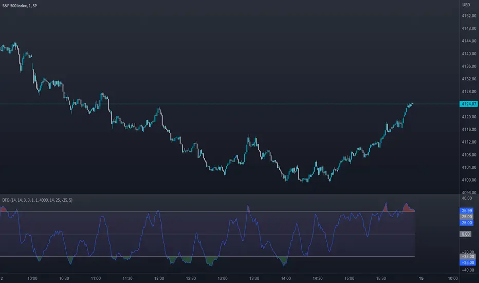
GKD-C QQE of Variety RSI [Loxx]Giga Kaleidoscope GKD-C QQE of Variety RSI is a Confirmation module included in Loxx's "Giga Kaleidoscope Modularized Trading System".
█ GKD-C QQE of Variety RSI
QQE: A Comprehensive Alternative to the Relative Strength Index
The Relative Strength Index (RSI) is a popular technical indicator that measures the speed and change of price movements to help traders identify potential trend reversals, overbought, and oversold conditions. Although the RSI is widely used, it has its limitations, and traders often seek alternative or complementary indicators to improve their market analysis. One such alternative is the Qualitative Quantitative Estimation (QQE) indicator, a comprehensive oscillator that combines the features of the RSI with additional smoothing and volatility adjustments. In the following, we will explore the QQE indicator, its calculation, and its potential benefits compared to using any type of RSI alone.
QQE Indicator
The QQE indicator was developed by an unknown author and is based on the RSI with additional modifications to enhance its performance. The QQE calculation involves three main steps:
1. The first step is to compute the RSI value for a specified period using the traditional RSI formula.
2. The second step is to apply a smoothing technique, such as the Wilder's smoothing or an exponential moving average (EMA), to the RSI value, resulting in the smoothed RSI.
3. The third step is to calculate the volatility-adjusted upper and lower bands (referred to as the QQE lines) around the smoothed RSI using an ATR-based (Average True Range) multiplier.
The QQE indicator is typically displayed as an oscillator with the smoothed RSI line in the middle and the upper and lower QQE lines acting as dynamic boundaries.
Comparison with the RSI
To better understand the potential benefits of the QQE indicator compared to using any type of RSI alone, let's examine its key features and how they may contribute to improved market analysis.
Advantages
1. The QQE indicator provides a more comprehensive view of the market by combining the strengths of the RSI with additional smoothing and volatility adjustments. This may result in a more reliable and accurate reflection of market conditions and price trends.
2. The smoothed RSI line in the QQE oscillator can help filter out noise and reduce the number of false signals often experienced when using the traditional RSI alone, making it easier for traders to identify genuine trend reversals and trading opportunities.
3. The dynamic QQE lines offer an additional layer of information by accounting for market volatility. This can help traders to better gauge the strength of price movements and identify potential support and resistance levels.
4. The QQE indicator can be used as a standalone tool or in combination with other technical indicators, providing traders with greater flexibility in their market analysis.
Disadvantages
1. The QQE indicator may be more complex to understand and implement than the traditional RSI due to the additional smoothing and volatility adjustments involved in its calculation.
2. As the QQE indicator is less widely known and used than the RSI, traders may find it more challenging to find resources and support for incorporating this indicator into their trading strategies.
Conclusion:
The QQE indicator is a versatile and comprehensive alternative to the traditional RSI, offering potential benefits in terms of noise reduction, volatility adjustment, and improved market analysis. However, it is important to recognize its limitations, such as increased complexity and limited resources compared to the RSI. Traders should carefully consider the potential advantages and drawbacks of using the QQE indicator before integrating it into their trading strategies. Ultimately, the choice between the QQE and any type of RSI will depend on individual traders' preferences and the specific market conditions they are analyzing.
This indicator includes 3 types of signals
1. Middle cross
2. Levels cross
3. Slow Trend cross
This indicator includes 9 types of RSI
1. Regular RSI
2. Slow RSI
3. Ehlers Smoothed RSI
4. Cutler's RSI or Rapid RSI
5. RSI T3
6. RSI DEMA
7. Harris' RSI
8. RSI TEMA
9. Jurik RSX
Regular RSI
The Relative Strength Index (RSI) is a widely used technical indicator in the field of financial market analysis. Developed by J. Welles Wilder Jr. in 1978, the RSI is a momentum oscillator that measures the speed and change of price movements. It helps traders identify potential trend reversals, overbought, and oversold conditions in a market.
The RSI is calculated based on the average gains and losses of an asset over a specified period, typically 14 days. The formula for calculating the RSI is as follows:
RSI = 100 - (100 / (1 + RS))
Where:
RS (Relative Strength) = Average gain over the specified period / Average loss over the specified period
The RSI ranges from 0 to 100, with values above 70 generally considered overbought (potentially indicating that the asset is overvalued and may experience a price decline) and values below 30 considered oversold (potentially indicating that the asset is undervalued and may experience a price increase).
Slow RSI
The Slow RSI is a variation of the standard RSI, which introduces a smoothing technique to the RSI calculation itself. The primary difference between the Slow RSI and the standard RSI lies in the calculation of the RSI value. In the Slow RSI, the current RSI value is calculated as a moving average of the previous RSI value and the standard RSI value for the current period.
The primary advantage of the Slow RSI is that it offers enhanced signal stability, reducing noise and potentially providing more reliable trading signals for traders.
Comparison with the original RSI
To better understand the potential advantages and disadvantages of the Slow RSI, it is essential to compare its performance against the original RSI.
Advantages
1. The Slow RSI provides enhanced signal stability by smoothing the RSI calculation, which can help traders better assess market conditions and identify potential overbought or oversold situations.
2. By offering more stable and reliable signals, the Slow RSI may improve the performance of trading strategies based on the RSI, especially in noisy or choppy market conditions.
Disadvantages
1. The smoothing technique employed by the Slow RSI may result in a slower response to changes in price momentum compared to the original RSI. This could lead to delayed signals for entering or exiting trades, which may not be ideal for short-term traders or fast-moving markets.
2. As the Slow RSI is less known and less widely used than the standard RSI, traders may find it more challenging to find resources and support for implementing this variation of the indicator.
The Slow RSI is an interesting modification of the standard RSI, offering potential benefits in terms of signal stability and reliability. However, it is crucial to recognize its limitations, such as a potentially slower response to changes in price momentum. Traders should carefully consider the potential advantages and drawbacks of using the Slow RSI compared to the original RSI before incorporating it into their trading strategies. Ultimately, the choice between the original RSI and the Slow RSI will depend on individual traders' preferences and the specific market conditions they are analyzing.
Ehlers Smoothed RSI
Ehlers Smoothed RSI is a variation of the standard RSI developed by John F. Ehlers, which introduces a smoothing technique to the price input data. The smoothing process involves averaging the current price with the previous two price values, which helps reduce noise and provide a more accurate representation of price momentum. The calculation of up and down price movements remains similar to the original RSI, but the smoothing technique alters the input data.
The primary advantage of Ehlers Smoothed RSI is that it reduces noise and offers a more accurate representation of price momentum, potentially providing more reliable signals for traders.
Comparison with the original RSI
To better understand the potential advantages and disadvantages of Ehlers Smoothed RSI, it is essential to compare its performance against the original RSI.
Advantages
1. Ehlers Smoothed RSI reduces noise by smoothing the price input data, which can help traders better assess market conditions and identify potential overbought or oversold situations.
2. By providing a more accurate representation of price momentum, Ehlers Smoothed RSI may offer more reliable signals for entering or exiting trades, potentially improving the performance of trading strategies based on the RSI.
Disadvantages
1. The smoothing technique employed by Ehlers Smoothed RSI may result in a slower response to changes in price momentum compared to the original RSI. This could lead to delayed signals for entering or exiting trades, which may not be ideal for short-term traders or fast-moving markets.
2. As Ehlers Smoothed RSI is less known and less widely used than the standard RSI, traders may find it more challenging to find resources and support for implementing this variation of the indicator.
Ehlers Smoothed RSI is an intriguing modification of the standard RSI, offering potential benefits in terms of noise reduction and accuracy. However, it is crucial to recognize its limitations, such as a potentially slower response to changes in price momentum. Traders should carefully consider the potential advantages and drawbacks of using Ehlers Smoothed RSI compared to the original RSI before incorporating it into their trading strategies. Ultimately, the choice between the original RSI and Ehlers Smoothed RSI will depend on individual traders' preferences and the specific market conditions they are analyzing.
Cutler's RSI or Rapid RSI
Cutler's RSI is a variation of the standard RSI, which modifies the calculation of average gains and losses. While the original RSI employs exponential moving averages (EMAs) for average gains and losses, Cutler's RSI utilizes simple moving averages (SMAs) instead. This change results in a slightly different behavior of the oscillator compared to the original RSI.
The primary advantage of Cutler's RSI is that it offers a simpler calculation method, which can potentially make it easier to understand and implement for traders. Additionally, by using SMAs, Cutler's RSI may provide a more consistent and stable representation of price momentum.
Comparison with the original RSI
It is essential to recognize the limitations and performance of Cutler's RSI compared to the original RSI to understand its potential advantages and disadvantages better.
Advantages
1. Cutler's RSI has a simpler calculation method, using SMAs instead of EMAs. This makes it easier to understand and implement for traders who prefer a more straightforward approach to technical analysis.
2. By using SMAs, Cutler's RSI may provide a more stable and consistent representation of price momentum, which can help traders better assess market conditions and identify potential overbought or oversold situations.
Disadvantages
1. The use of SMAs in Cutler's RSI may result in a slower response to changes in price momentum compared to the original RSI. This could lead to delayed signals for entering or exiting trades, which may not be ideal for short-term traders or fast-moving markets.
2. As Cutler's RSI is less known and less widely used than the standard RSI, it may be more challenging to find resources and support for implementing this variation of the indicator.
Cutler's RSI is an interesting modification of the standard RSI, offering potential benefits in terms of simplicity and stability. However, it is crucial to recognize its limitations, such as a potentially slower response to changes in price momentum. Traders should carefully consider the potential advantages and drawbacks of using Cutler's RSI compared to the original RSI before incorporating it into their trading strategies. Ultimately, the choice between the original RSI and Cutler's RSI will depend on individual traders' preferences and the specific market conditions they are analyzing.
RSI T3
The T3 RSI is a variation of the standard RSI that introduces the Triple Smoothed Exponential Moving Average (T3) into the calculation process. The primary difference between the T3 RSI and the standard RSI lies in the calculation of the average gains and losses. Instead of using simple moving averages or exponential moving averages, the T3 RSI utilizes T3 to calculate the average gains and losses for up and down price movements.
The primary advantage of the T3 RSI is that it offers enhanced responsiveness and accuracy compared to the original RSI, potentially providing more reliable trading signals for traders.
Comparison with the original RSI
To better understand the potential advantages and disadvantages of the T3 RSI, it is essential to compare its performance against the original RSI.
Advantages
1. The T3 RSI provides enhanced responsiveness and accuracy by incorporating the Triple Smoothed Exponential Moving Average into the calculation of average gains and losses. This can help traders better assess market conditions and identify potential overbought or oversold situations.
2. By offering more responsive and accurate signals, the T3 RSI may improve the performance of trading strategies based on the RSI, especially in fast-moving markets or during periods of high price volatility.
Disadvantages
1. The T3 RSI's increased responsiveness may result in more frequent trading signals, which could lead to higher trading costs or a higher likelihood of false signals.
2. As the T3 RSI is less known and less widely used than the standard RSI, traders may find it more challenging to find resources and support for implementing this variation of the indicator.
The T3 RSI is an innovative modification of the standard RSI, offering potential benefits in terms of responsiveness and accuracy. However, it is crucial to recognize its limitations, such as a potentially higher likelihood of false signals due to increased responsiveness. Traders should carefully consider the potential advantages and drawbacks of using the T3 RSI compared to the original RSI before incorporating it into their trading strategies. Ultimately, the choice between the original RSI and the T3 RSI will depend on individual traders' preferences and the specific market conditions they are analyzing.
RSI DEMA
The DEMA RSI is a variation of the standard RSI that introduces the Double Exponential Moving Average (DEMA) into the calculation process. The primary difference between the DEMA RSI and the standard RSI lies in the calculation of the average gains and losses. Instead of using simple moving averages or exponential moving averages, the DEMA RSI utilizes DEMA to calculate the average gains and losses for up and down price movements.
The primary advantage of the DEMA RSI is that it offers enhanced responsiveness and accuracy compared to the original RSI, potentially providing more reliable trading signals for traders.
Comparison with the original RSI
To better understand the potential advantages and disadvantages of the DEMA RSI, it is essential to compare its performance against the original RSI.
Advantages
1. The DEMA RSI provides enhanced responsiveness and accuracy by incorporating the Double Exponential Moving Average into the calculation of average gains and losses. This can help traders better assess market conditions and identify potential overbought or oversold situations.
2. By offering more responsive and accurate signals, the DEMA RSI may improve the performance of trading strategies based on the RSI, especially in fast-moving markets or during periods of high price volatility.
Disadvantages
1. The DEMA RSI's increased responsiveness may result in more frequent trading signals, which could lead to higher trading costs or a higher likelihood of false signals.
2. As the DEMA RSI is less known and less widely used than the standard RSI, traders may find it more challenging to find resources and support for implementing this variation of the indicator.
The DEMA RSI is an innovative modification of the standard RSI, offering potential benefits in terms of responsiveness and accuracy. However, it is crucial to recognize its limitations, such as a potentially higher likelihood of false signals due to increased responsiveness. Traders should carefully consider the potential advantages and drawbacks of using the DEMA RSI compared to the original RSI before incorporating it into their trading strategies. Ultimately, the choice between the original RSI and the DEMA RSI will depend on individual traders' preferences and the specific market conditions they are analyzing.
Harris' RSI
Harris' RSI is a variation of the standard RSI, designed to address some of its limitations and improve its performance in detecting potential trend reversals and filtering out noise. The key difference between the Harris' RSI and the standard RSI lies in the calculation of average gains and losses. While the standard RSI calculation uses exponential moving averages (EMAs) of gains and losses, Harris' RSI uses a different approach to compute the average gains and losses based on the number of up and down price movements.
The primary advantage of Harris' RSI is that it aims to provide a more adaptive and responsive indicator, making it better suited for detecting potential trend reversals and filtering out noise in the market. By taking into account the number of up and down price movements, Harris' RSI can be more sensitive to changes in the trend, potentially providing earlier signals for entering or exiting trades.
Comparison with the original RSI
While Harris' RSI offers potential improvements over the standard RSI, it is essential to recognize its limitations and compare its performance against the original RSI.
Advantages
1. Harris' RSI can potentially provide earlier signals for trend reversals due to its sensitivity to the number of up and down price movements. This can help traders to identify better entry and exit points in the market.
2. By focusing on the number of up and down price movements, Harris' RSI can filter out noise in the market, reducing the likelihood of false signals that may lead to losing trades.
Disadvantages
1. The increased sensitivity of Harris' RSI to price movements can lead to more frequent signals, which may result in overtrading and increased trading costs.
2. Harris' RSI is less known and less widely used than the standard RSI, which may make it more challenging to find resources and support for implementing this variation of the indicator.
Harris' RSI is an interesting variation of the standard RSI, offering potential advantages in detecting trend reversals and filtering out noise. However, like any technical indicator, it has its limitations and may not be suitable for all trading styles or market conditions. Traders should carefully consider the potential benefits and drawbacks of using Harris' RSI compared to the original RSI before incorporating it into their trading strategies. Ultimately, the choice between the original RSI and Harris' RSI will depend on individual traders' preferences and the specific market conditions they are analyzing.
RSI TEMA
The TEMA RSI is a variation of the standard RSI that introduces the Triple Exponential Moving Average (TEMA) into the calculation process. The primary difference between the TEMA RSI and the standard RSI lies in the calculation of the average gains and losses. Instead of using simple moving averages or exponential moving averages, the TEMA RSI utilizes TEMA to calculate the average gains and losses for up and down price movements.
The primary advantage of the TEMA RSI is that it offers enhanced responsiveness and accuracy compared to the original RSI, potentially providing more reliable trading signals for traders.
Comparison with the original RSI
To better understand the potential advantages and disadvantages of the TEMA RSI, it is essential to compare its performance against the original RSI.
Advantages
1. The TEMA RSI provides enhanced responsiveness and accuracy by incorporating the Triple Exponential Moving Average into the calculation of average gains and losses. This can help traders better assess market conditions and identify potential overbought or oversold situations.
2. By offering more responsive and accurate signals, the TEMA RSI may improve the performance of trading strategies based on the RSI, especially in fast-moving markets or during periods of high price volatility.
Disadvantages
1. The TEMA RSI's increased responsiveness may result in more frequent trading signals, which could lead to higher trading costs or a higher likelihood of false signals.
2. As the TEMA RSI is less known and less widely used than the standard RSI, traders may find it more challenging to find resources and support for implementing this variation of the indicator.
The TEMA RSI is an innovative modification of the standard RSI, offering potential benefits in terms of responsiveness and accuracy. However, it is crucial to recognize its limitations, such as a potentially higher likelihood of false signals due to increased responsiveness. Traders should carefully consider the potential advantages and drawbacks of using the TEMA RSI compared to the original RSI before incorporating it into their trading strategies. Ultimately, the choice between the original RSI and the TEMA RSI will depend on individual traders' preferences and the specific market conditions they are analyzing.
Jurik RSX
The Jurik RSX, developed by Mark Jurik, is a variation of the standard RSI that aims to provide a smoother and more responsive indicator by applying a unique smoothing algorithm based on a series of recursive calculations. The Jurik RSX calculates the price momentum (mom) and the absolute price momentum (moa) using a three-stage filtering process, which ultimately results in a smoother and more responsive output compared to the original RSI.
Comparison with the original RSI
To better understand the potential benefits and drawbacks of the Jurik RSX, it is essential to compare its performance against the original RSI.
Advantages
1. The Jurik RSX offers enhanced responsiveness and smoothness due to its unique recursive filtering process, allowing traders to better identify potential trend reversals, overbought, and oversold conditions.
2. The improved responsiveness of the Jurik RSX may result in more timely trading signals, helping traders to capitalize on opportunities more effectively, especially in fast-moving markets or during periods of high price volatility.
Disadvantages
1. The increased complexity of the Jurik RSX calculation may make it more challenging for traders to understand and implement compared to the original RSI.
2. As the Jurik RSX is less known and less widely used than the standard RSI, traders may find it more difficult to find resources and support for implementing this variation of the indicator.
The Jurik RSX is an innovative modification of the standard RSI, offering potential benefits in terms of responsiveness and smoothness. However, it is crucial to recognize its limitations, such as increased complexity and limited resources compared to the original RSI. Traders should carefully consider the potential advantages and drawbacks of using the Jurik RSX before incorporating it into their trading strategies. Ultimately, the choice between the original RSI and the Jurik RSX will depend on individual traders' preferences and the specific market conditions they are analyzing.
Additional Features
This indicator allows you to select from 33 source types. They are as follows:
Close
Open
High
Low
Median
Typical
Weighted
Average
Average Median Body
Trend Biased
Trend Biased (Extreme)
HA Close
HA Open
HA High
HA Low
HA Median
HA Typical
HA Weighted
HA Average
HA Average Median Body
HA Trend Biased
HA Trend Biased (Extreme)
HAB Close
HAB Open
HAB High
HAB Low
HAB Median
HAB Typical
HAB Weighted
HAB Average
HAB Average Median Body
HAB Trend Biased
HAB Trend Biased (Extreme)
What are Heiken Ashi "better" candles?
Heiken Ashi "better" candles are a modified version of the standard Heiken Ashi candles, which are a popular charting technique used in technical analysis. Heiken Ashi candles help traders identify trends and potential reversal points by smoothing out price data and reducing market noise. The "better formula" was proposed by Sebastian Schmidt in an article published by BNP Paribas in Warrants & Zertifikate, a German magazine, in August 2004. The aim of this formula is to further improve the smoothing of the Heiken Ashi chart and enhance its effectiveness in identifying trends and reversals.
Standard Heiken Ashi candles are calculated using the following formulas:
Heiken Ashi Close = (Open + High + Low + Close) / 4
Heiken Ashi Open = (Previous Heiken Ashi Open + Previous Heiken Ashi Close) / 2
Heiken Ashi High = Max (High, Heiken Ashi Open, Heiken Ashi Close)
Heiken Ashi Low = Min (Low, Heiken Ashi Open, Heiken Ashi Close)
The "better formula" modifies the standard Heiken Ashi calculation by incorporating additional smoothing, which can help reduce noise and make it easier to identify trends and reversals. The modified formulas for Heiken Ashi "better" candles are as follows:
Better Heiken Ashi Close = (Open + High + Low + Close) / 4
Better Heiken Ashi Open = (Previous Better Heiken Ashi Open + Previous Better Heiken Ashi Close) / 2
Better Heiken Ashi High = Max (High, Better Heiken Ashi Open, Better Heiken Ashi Close)
Better Heiken Ashi Low = Min (Low, Better Heiken Ashi Open, Better Heiken Ashi Close)
Smoothing Factor = 2 / (N + 1), where N is the chosen period for smoothing
Smoothed Better Heiken Ashi Open = (Better Heiken Ashi Open * Smoothing Factor) + (Previous Smoothed Better Heiken Ashi Open * (1 - Smoothing Factor))
Smoothed Better Heiken Ashi Close = (Better Heiken Ashi Close * Smoothing Factor) + (Previous Smoothed Better Heiken Ashi Close * (1 - Smoothing Factor))
The smoothed Better Heiken Ashi Open and Close values are then used to calculate the smoothed Better Heiken Ashi High and Low values, resulting in "better" candles that provide a clearer representation of the market trend and potential reversal points.
It's important to note that, like any other technical analysis tool, Heiken Ashi "better" candles are not foolproof and should be used in conjunction with other indicators and analysis techniques to make well-informed trading decisions.
Heiken Ashi "better" candles, as mentioned previously, provide a clearer representation of market trends and potential reversal points by reducing noise and smoothing out price data. When using these candles in conjunction with other technical analysis tools and indicators, traders can gain valuable insights into market behavior and make more informed decisions.
To effectively use Heiken Ashi "better" candles in your trading strategy, consider the following tips:
Trend Identification: Heiken Ashi "better" candles can help you identify the prevailing trend in the market. When the majority of the candles are green (or another color, depending on your chart settings) and there are no or few lower wicks, it may indicate a strong uptrend. Conversely, when the majority of the candles are red (or another color) and there are no or few upper wicks, it may signal a strong downtrend.
Trend Reversals: Look for potential trend reversals when a change in the color of the candles occurs, especially when accompanied by longer wicks. For example, if a green candle with a long lower wick is followed by a red candle, it could indicate a bearish reversal. Similarly, a red candle with a long upper wick followed by a green candle may suggest a bullish reversal.
Support and Resistance: You can use Heiken Ashi "better" candles to identify potential support and resistance levels. When the candles are consistently moving in one direction and then suddenly change color with longer wicks, it could indicate the presence of a support or resistance level.
Stop-Loss and Take-Profit: Using Heiken Ashi "better" candles can help you manage risk by determining optimal stop-loss and take-profit levels. For instance, you can place your stop-loss below the low of the most recent green candle in an uptrend or above the high of the most recent red candle in a downtrend.
Confirming Signals: Heiken Ashi "better" candles should be used in conjunction with other technical indicators, such as moving averages, oscillators, or chart patterns, to confirm signals and improve the accuracy of your analysis.
In this implementation, you have the choice of AMA, KAMA, or T3 smoothing. These are as follows:
Kaufman Adaptive Moving Average (KAMA)
The Kaufman Adaptive Moving Average (KAMA) is a type of adaptive moving average used in technical analysis to smooth out price fluctuations and identify trends. The KAMA adjusts its smoothing factor based on the market's volatility, making it more responsive in volatile markets and smoother in calm markets. The KAMA is calculated using three different efficiency ratios that determine the appropriate smoothing factor for the current market conditions. These ratios are based on the noise level of the market, the speed at which the market is moving, and the length of the moving average. The KAMA is a popular choice among traders who prefer to use adaptive indicators to identify trends and potential reversals.
Adaptive Moving Average
The Adaptive Moving Average (AMA) is a type of moving average that adjusts its sensitivity to price movements based on market conditions. It uses a ratio between the current price and the highest and lowest prices over a certain lookback period to determine its level of smoothing. The AMA can help reduce lag and increase responsiveness to changes in trend direction, making it useful for traders who want to follow trends while avoiding false signals. The AMA is calculated by multiplying a smoothing constant with the difference between the current price and the previous AMA value, then adding the result to the previous AMA value.
T3
The T3 moving average is a type of technical indicator used in financial analysis to identify trends in price movements. It is similar to the Exponential Moving Average (EMA) and the Double Exponential Moving Average (DEMA), but uses a different smoothing algorithm.
The T3 moving average is calculated using a series of exponential moving averages that are designed to filter out noise and smooth the data. The resulting smoothed data is then weighted with a non-linear function to produce a final output that is more responsive to changes in trend direction.
The T3 moving average can be customized by adjusting the length of the moving average, as well as the weighting function used to smooth the data. It is commonly used in conjunction with other technical indicators as part of a larger trading strategy.
█ Giga Kaleidoscope Modularized Trading System
Core components of an NNFX algorithmic trading strategy
The NNFX algorithm is built on the principles of trend, momentum, and volatility. There are six core components in the NNFX trading algorithm:
1. Volatility - price volatility; e.g., Average True Range, True Range Double, Close-to-Close, etc.
2. Baseline - a moving average to identify price trend
3. Confirmation 1 - a technical indicator used to identify trends
4. Confirmation 2 - a technical indicator used to identify trends
5. Continuation - a technical indicator used to identify trends
6. Volatility/Volume - a technical indicator used to identify volatility/volume breakouts/breakdown
7. Exit - a technical indicator used to determine when a trend is exhausted
What is Volatility in the NNFX trading system?
In the NNFX (No Nonsense Forex) trading system, ATR (Average True Range) is typically used to measure the volatility of an asset. It is used as a part of the system to help determine the appropriate stop loss and take profit levels for a trade. ATR is calculated by taking the average of the true range values over a specified period.
True range is calculated as the maximum of the following values:
-Current high minus the current low
-Absolute value of the current high minus the previous close
-Absolute value of the current low minus the previous close
ATR is a dynamic indicator that changes with changes in volatility. As volatility increases, the value of ATR increases, and as volatility decreases, the value of ATR decreases. By using ATR in NNFX system, traders can adjust their stop loss and take profit levels according to the volatility of the asset being traded. This helps to ensure that the trade is given enough room to move, while also minimizing potential losses.
Other types of volatility include True Range Double (TRD), Close-to-Close, and Garman-Klass
What is a Baseline indicator?
The baseline is essentially a moving average, and is used to determine the overall direction of the market.
The baseline in the NNFX system is used to filter out trades that are not in line with the long-term trend of the market. The baseline is plotted on the chart along with other indicators, such as the Moving Average (MA), the Relative Strength Index (RSI), and the Average True Range (ATR).
Trades are only taken when the price is in the same direction as the baseline. For example, if the baseline is sloping upwards, only long trades are taken, and if the baseline is sloping downwards, only short trades are taken. This approach helps to ensure that trades are in line with the overall trend of the market, and reduces the risk of entering trades that are likely to fail.
By using a baseline in the NNFX system, traders can have a clear reference point for determining the overall trend of the market, and can make more informed trading decisions. The baseline helps to filter out noise and false signals, and ensures that trades are taken in the direction of the long-term trend.
What is a Confirmation indicator?
Confirmation indicators are technical indicators that are used to confirm the signals generated by primary indicators. Primary indicators are the core indicators used in the NNFX system, such as the Average True Range (ATR), the Moving Average (MA), and the Relative Strength Index (RSI).
The purpose of the confirmation indicators is to reduce false signals and improve the accuracy of the trading system. They are designed to confirm the signals generated by the primary indicators by providing additional information about the strength and direction of the trend.
Some examples of confirmation indicators that may be used in the NNFX system include the Bollinger Bands, the MACD (Moving Average Convergence Divergence), and the MACD Oscillator. These indicators can provide information about the volatility, momentum, and trend strength of the market, and can be used to confirm the signals generated by the primary indicators.
In the NNFX system, confirmation indicators are used in combination with primary indicators and other filters to create a trading system that is robust and reliable. By using multiple indicators to confirm trading signals, the system aims to reduce the risk of false signals and improve the overall profitability of the trades.
What is a Continuation indicator?
In the NNFX (No Nonsense Forex) trading system, a continuation indicator is a technical indicator that is used to confirm a current trend and predict that the trend is likely to continue in the same direction. A continuation indicator is typically used in conjunction with other indicators in the system, such as a baseline indicator, to provide a comprehensive trading strategy.
What is a Volatility/Volume indicator?
Volume indicators, such as the On Balance Volume (OBV), the Chaikin Money Flow (CMF), or the Volume Price Trend (VPT), are used to measure the amount of buying and selling activity in a market. They are based on the trading volume of the market, and can provide information about the strength of the trend. In the NNFX system, volume indicators are used to confirm trading signals generated by the Moving Average and the Relative Strength Index. Volatility indicators include Average Direction Index, Waddah Attar, and Volatility Ratio. In the NNFX trading system, volatility is a proxy for volume and vice versa.
By using volume indicators as confirmation tools, the NNFX trading system aims to reduce the risk of false signals and improve the overall profitability of trades. These indicators can provide additional information about the market that is not captured by the primary indicators, and can help traders to make more informed trading decisions. In addition, volume indicators can be used to identify potential changes in market trends and to confirm the strength of price movements.
What is an Exit indicator?
The exit indicator is used in conjunction with other indicators in the system, such as the Moving Average (MA), the Relative Strength Index (RSI), and the Average True Range (ATR), to provide a comprehensive trading strategy.
The exit indicator in the NNFX system can be any technical indicator that is deemed effective at identifying optimal exit points. Examples of exit indicators that are commonly used include the Parabolic SAR, the Average Directional Index (ADX), and the Chandelier Exit.
The purpose of the exit indicator is to identify when a trend is likely to reverse or when the market conditions have changed, signaling the need to exit a trade. By using an exit indicator, traders can manage their risk and prevent significant losses.
In the NNFX system, the exit indicator is used in conjunction with a stop loss and a take profit order to maximize profits and minimize losses. The stop loss order is used to limit the amount of loss that can be incurred if the trade goes against the trader, while the take profit order is used to lock in profits when the trade is moving in the trader's favor.
Overall, the use of an exit indicator in the NNFX trading system is an important component of a comprehensive trading strategy. It allows traders to manage their risk effectively and improve the profitability of their trades by exiting at the right time.
How does Loxx's GKD (Giga Kaleidoscope Modularized Trading System) implement the NNFX algorithm outlined above?
Loxx's GKD v1.0 system has five types of modules (indicators/strategies). These modules are:
1. GKD-BT - Backtesting module (Volatility, Number 1 in the NNFX algorithm)
2. GKD-B - Baseline module (Baseline and Volatility/Volume, Numbers 1 and 2 in the NNFX algorithm)
3. GKD-C - Confirmation 1/2 and Continuation module (Confirmation 1/2 and Continuation, Numbers 3, 4, and 5 in the NNFX algorithm)
4. GKD-V - Volatility/Volume module (Confirmation 1/2, Number 6 in the NNFX algorithm)
5. GKD-E - Exit module (Exit, Number 7 in the NNFX algorithm)
(additional module types will added in future releases)
Each module interacts with every module by passing data between modules. Data is passed between each module as described below:
GKD-B => GKD-V => GKD-C(1) => GKD-C(2) => GKD-C(Continuation) => GKD-E => GKD-BT
That is, the Baseline indicator passes its data to Volatility/Volume. The Volatility/Volume indicator passes its values to the Confirmation 1 indicator. The Confirmation 1 indicator passes its values to the Confirmation 2 indicator. The Confirmation 2 indicator passes its values to the Continuation indicator. The Continuation indicator passes its values to the Exit indicator, and finally, the Exit indicator passes its values to the Backtest strategy.
This chaining of indicators requires that each module conform to Loxx's GKD protocol, therefore allowing for the testing of every possible combination of technical indicators that make up the six components of the NNFX algorithm.
What does the application of the GKD trading system look like?
Example trading system:
Backtest: Strategy with 1-3 take profits, trailing stop loss, multiple types of PnL volatility, and 2 backtesting styles
Baseline: Hull Moving Average
Volatility/Volume: Hurst Exponent
Confirmation 1: QQE of Variety RSI as shown on the chart above
Confirmation 2: Williams Percent Range
Continuation: QQE of Variety RSI
Exit: Rex Oscillator
Each GKD indicator is denoted with a module identifier of either: GKD-BT, GKD-B, GKD-C, GKD-V, or GKD-E. This allows traders to understand to which module each indicator belongs and where each indicator fits into the GKD protocol chain.
Giga Kaleidoscope Modularized Trading System Signals (based on the NNFX algorithm)
Standard Entry
1. GKD-C Confirmation 1 Signal
2. GKD-B Baseline agrees
3. Price is within a range of 0.2x Volatility and 1.0x Volatility of the Goldie Locks Mean
4. GKD-C Confirmation 2 agrees
5. GKD-V Volatility/Volume agrees
Baseline Entry
1. GKD-B Baseline signal
2. GKD-C Confirmation 1 agrees
3. Price is within a range of 0.2x Volatility and 1.0x Volatility of the Goldie Locks Mean
4. GKD-C Confirmation 2 agrees
5. GKD-V Volatility/Volume agrees
6. GKD-C Confirmation 1 signal was less than 7 candles prior
Volatility/Volume Entry
1. GKD-V Volatility/Volume signal
2. GKD-C Confirmation 1 agrees
3. Price is within a range of 0.2x Volatility and 1.0x Volatility of the Goldie Locks Mean
4. GKD-C Confirmation 2 agrees
5. GKD-B Baseline agrees
6. GKD-C Confirmation 1 signal was less than 7 candles prior
Continuation Entry
1. Standard Entry, Baseline Entry, or Pullback; entry triggered previously
2. GKD-B Baseline hasn't crossed since entry signal trigger
3. GKD-C Confirmation Continuation Indicator signals
4. GKD-C Confirmation 1 agrees
5. GKD-B Baseline agrees
6. GKD-C Confirmation 2 agrees
1-Candle Rule Standard Entry
1. GKD-C Confirmation 1 signal
2. GKD-B Baseline agrees
3. Price is within a range of 0.2x Volatility and 1.0x Volatility of the Goldie Locks Mean
Next Candle:
1. Price retraced (Long: close < close or Short: close > close )
2. GKD-B Baseline agrees
3. GKD-C Confirmation 1 agrees
4. GKD-C Confirmation 2 agrees
5. GKD-V Volatility/Volume agrees
1-Candle Rule Baseline Entry
1. GKD-B Baseline signal
2. GKD-C Confirmation 1 agrees
3. Price is within a range of 0.2x Volatility and 1.0x Volatility of the Goldie Locks Mean
4. GKD-C Confirmation 1 signal was less than 7 candles prior
Next Candle:
1. Price retraced (Long: close < close or Short: close > close )
2. GKD-B Baseline agrees
3. GKD-C Confirmation 1 agrees
4. GKD-C Confirmation 2 agrees
5. GKD-V Volatility/Volume Agrees
1-Candle Rule Volatility/Volume Entry
1. GKD-V Volatility/Volume signal
2. GKD-C Confirmation 1 agrees
3. Price is within a range of 0.2x Volatility and 1.0x Volatility of the Goldie Locks Mean
4. GKD-C Confirmation 1 signal was less than 7 candles prior
Next Candle:
1. Price retraced (Long: close < close or Short: close > close)
2. GKD-B Volatility/Volume agrees
3. GKD-C Confirmation 1 agrees
4. GKD-C Confirmation 2 agrees
5. GKD-B Baseline agrees
PullBack Entry
1. GKD-B Baseline signal
2. GKD-C Confirmation 1 agrees
3. Price is beyond 1.0x Volatility of Baseline
Next Candle:
1. Price is within a range of 0.2x Volatility and 1.0x Volatility of the Goldie Locks Mean
2. GKD-C Confirmation 1 agrees
3. GKD-C Confirmation 2 agrees
4. GKD-V Volatility/Volume Agrees
]█ Setting up the GKD
The GKD system involves chaining indicators together. These are the steps to set this up.
Use a GKD-C indicator alone on a chart
1. Inside the GKD-C indicator, change the "Confirmation Type" setting to "Solo Confirmation Simple"
Use a GKD-V indicator alone on a chart
**nothing, it's already useable on the chart without any settings changes
Use a GKD-B indicator alone on a chart
**nothing, it's already useable on the chart without any settings changes
Baseline (Baseline, Backtest)
1. Import the GKD-B Baseline into the GKD-BT Backtest: "Input into Volatility/Volume or Backtest (Baseline testing)"
2. Inside the GKD-BT Backtest, change the setting "Backtest Special" to "Baseline"
Volatility/Volume (Volatility/Volume, Backte st)
1. Inside the GKD-V indicator, change the "Testing Type" setting to "Solo"
2. Inside the GKD-V indicator, change the "Signal Type" setting to "Crossing" (neither traditional nor both can be backtested)
3. Import the GKD-V indicator into the GKD-BT Backtest: "Input into C1 or Backtest"
4. Inside the GKD-BT Backtest, change the setting "Backtest Special" to "Volatility/Volume"
5. Inside the GKD-BT Backtest, a) change the setting "Backtest Type" to "Trading" if using a directional GKD-V indicator; or, b) change the setting "Backtest Type" to "Full" if using a directional or non-directional GKD-V indicator (non-directional GKD-V can only test Longs and Shorts separately)
6. If "Backtest Type" is set to "Full": Inside the GKD-BT Backtest, change the setting "Backtest Side" to "Long" or "Short
7. If "Backtest Type" is set to "Full": To allow the system to open multiple orders at one time so you test all Longs or Shorts, open the GKD-BT Backtest, click the tab "Properties" and then insert a value of something like 10 orders into the "Pyramiding" settings. This will allow 10 orders to be opened at one time which should be enough to catch all possible Longs or Shorts.
Solo Confirmation Simple (Confirmation, Backtest)
1. Inside the GKD-C indicator, change the "Confirmation Type" setting to "Solo Confirmation Simple"
1. Import the GKD-C indicator into the GKD-BT Backtest: "Input into Backtest"
2. Inside the GKD-BT Backtest, change the setting "Backtest Special" to "Solo Confirmation Simple"
Solo Confirmation Complex without Exits (Baseline, Volatility/Volume, Confirmation, Backtest)
1. Inside the GKD-V indicator, change the "Testing Type" setting to "Chained"
2. Import the GKD-B Baseline into the GKD-V indicator: "Input into Volatility/Volume or Backtest (Baseline testing)"
3. Inside the GKD-C indicator, change the "Confirmation Type" setting to "Solo Confirmation Complex"
4. Import the GKD-V indicator into the GKD-C indicator: "Input into C1 or Backtest"
5. Inside the GKD-BT Backtest, change the setting "Backtest Special" to "GKD Full wo/ Exits"
6. Import the GKD-C into the GKD-BT Backtest: "Input into Exit or Backtest"
Solo Confirmation Complex with Exits (Baseline, Volatility/Volume, Confirmation, Exit, Backtest)
1. Inside the GKD-V indicator, change the "Testing Type" setting to "Chained"
2. Import the GKD-B Baseline into the GKD-V indicator: "Input into Volatility/Volume or Backtest (Baseline testing)"
3. Inside the GKD-C indicator, change the "Confirmation Type" setting to "Solo Confirmation Complex"
4. Import the GKD-V indicator into the GKD-C indicator: "Input into C1 or Backtest"
5. Import the GKD-C indicator into the GKD-E indicator: "Input into Exit"
6. Inside the GKD-BT Backtest, change the setting "Backtest Special" to "GKD Full w/ Exits"
7. Import the GKD-E into the GKD-BT Backtest: "Input into Backtest"
Full GKD without Exits (Baseline, Volatility/Volume, Confirmation 1, Confirmation 2, Continuation, Backtest)
1. Inside the GKD-V indicator, change the "Testing Type" setting to "Chained"
2. Import the GKD-B Baseline into the GKD-V indicator: "Input into Volatility/Volume or Backtest (Baseline testing)"
3. Inside the GKD-C 1 indicator, change the "Confirmation Type" setting to "Confirmation 1"
4. Import the GKD-V indicator into the GKD-C 1 indicator: "Input into C1 or Backtest"
5. Inside the GKD-C 2 indicator, change the "Confirmation Type" setting to "Confirmation 2"
6. Import the GKD-C 1 indicator into the GKD-C 2 indicator: "Input into C2"
7. Inside the GKD-C Continuation indicator, change the "Confirmation Type" setting to "Continuation"
8. Inside the GKD-BT Backtest, change the setting "Backtest Special" to "GKD Full wo/ Exits"
9. Import the GKD-E into the GKD-BT Backtest: "Input into Exit or Backtest"
Full GKD with Exits (Baseline, Volatility/Volume, Confirmation 1, Confirmation 2, Continuation, Exit, Backtest)
1. Inside the GKD-V indicator, change the "Testing Type" setting to "Chained"
2. Import the GKD-B Baseline into the GKD-V indicator: "Input into Volatility/Volume or Backtest (Baseline testing)"
3. Inside the GKD-C 1 indicator, change the "Confirmation Type" setting to "Confirmation 1"
4. Import the GKD-V indicator into the GKD-C 1 indicator: "Input into C1 or Backtest"
5. Inside the GKD-C 2 indicator, change the "Confirmation Type" setting to "Confirmation 2"
6. Import the GKD-C 1 indicator into the GKD-C 2 indicator: "Input into C2"
7. Inside the GKD-C Continuation indicator, change the "Confirmation Type" setting to "Continuation"
8. Import the GKD-C Continuation indicator into the GKD-E indicator: "Input into Exit"
9. Inside the GKD-BT Backtest, change the setting "Backtest Special" to "GKD Full w/ Exits"
10. Import the GKD-E into the GKD-BT Backtest: "Input into Backtest"
Baseline + Volatility/Volume (Baseline, Volatility/Volume, Backtest)
1. Inside the GKD-V indicator, change the "Testing Type" setting to "Baseline + Volatility/Volume"
2. Inside the GKD-V indicator, make sure the "Signal Type" setting is set to "Traditional"
3. Import the GKD-B Baseline into the GKD-V indicator: "Input into Volatility/Volume or Backtest (Baseline testing)"
4. Inside the GKD-BT Backtest, change the setting "Backtest Special" to "Baseline + Volatility/Volume"
5. Import the GKD-V into the GKD-BT Backtest: "Input into C1 or Backtest"
6. Inside the GKD-BT Backtest, change the setting "Backtest Type" to "Full". For this backtest, you must test Longs and Shorts separately
7. To allow the system to open multiple orders at one time so you can test all Longs or Shorts, open the GKD-BT Backtest, click the tab "Properties" and then insert a value of something like 10 orders into the "Pyramiding" settings. This will allow 10 orders to be opened at one time which should be enough to catch all possible Longs or Shorts.
Requirements
Inputs
Confirmation 1: GKD-V Volatility / Volume indicator
Confirmation 2: GKD-C Confirmation indicator
Continuation: GKD-C Confirmation indicator
Solo Confirmation Simple: GKD-B Baseline
Solo Confirmation Complex: GKD-V Volatility / Volume indicator
Solo Confirmation Super Complex: GKD-V Volatility / Volume indicator
Stacked 1: None
Stacked 2+: GKD-C, GKD-V, or GKD-B Stacked 1
Outputs
Confirmation 1: GKD-C Confirmation 2 indicator
Confirmation 2: GKD-C Continuation indicator
Continuation: GKD-E Exit indicator
Solo Confirmation Simple: GKD-BT Backtest
Solo Confirmation Complex: GKD-BT Backtest or GKD-E Exit indicator
Solo Confirmation Super Complex: GKD-C Continuation indicator
Stacked 1: GKD-C, GKD-V, or GKD-B Stacked 2+
Stacked 2+: GKD-C, GKD-V, or GKD-B Stacked 2+ or GKD-BT Backtest
Additional features will be added in future releases.
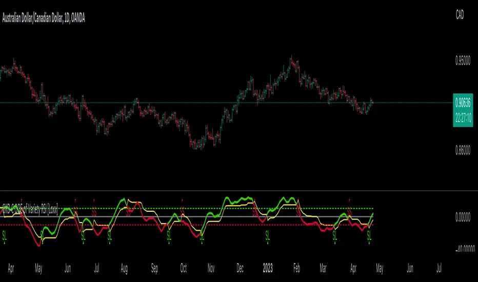
GKD-C RSI DEMA [Loxx]Giga Kaleidoscope GKD-C RSI DEMA is a Confirmation module included in Loxx's "Giga Kaleidoscope Modularized Trading System".
█ GKD-C RSI DEMA
Exploring RSI-DEMA: A Novel Indicator for Technical Analysis in Trading
The world of trading has evolved considerably with the advent of technology and the development of various technical analysis tools. These tools assist traders in making informed decisions based on the historical price movements of financial instruments. One such tool is the Relative Strength Index (RSI), which has been widely used to gauge the momentum of price movements. However, the following explores a new variation of RSI, calculated using the Double Exponential Moving Average (DEMA), which we will refer to as RSI-DEMA.
Background on RSI
The Relative Strength Index (RSI) is a momentum oscillator developed by J. Welles Wilder in 1978. It measures the speed and change of price movements, oscillating between 0 and 100. The RSI is typically used to identify overbought or oversold conditions in a market. An RSI value above 70 suggests an overbought condition, whereas a value below 30 indicates an oversold condition. This information can be valuable for traders in determining potential entry and exit points.
Introducing RSI-DEMA
The RSI-DEMA is a modified version of the traditional RSI that incorporates the Double Exponential Moving Average (DEMA) in its calculation. DEMA, developed by Patrick Mulloy, is a type of moving average that reacts more quickly to recent price changes compared to other moving averages like Simple Moving Average (SMA) and Exponential Moving Average (EMA). By combining RSI with DEMA, the RSI-DEMA aims to provide a more sensitive and responsive momentum oscillator for traders to analyze market conditions.
RSI-DEMA Calculation
The RSI-DEMA formula calculates the RSI-DEMA value for a given input price (src) and period (per). The first step is to compute the alpha value, which is inversely proportional to the square root of the period. Next, the price change is calculated and separated into positive and negative changes. These changes are then smoothed using the DEMA method, which involves two stages of exponential smoothing.
Finally, the smoothed positive and negative changes are divided, and the result is scaled by 50 to obtain the RSI-DEMA value, which oscillates between 0 and 100. This value provides insight into the strength of the price momentum and can be used similarly to the traditional RSI to identify overbought and oversold conditions in the market.
Advantages of RSI-DEMA
The primary advantage of RSI-DEMA over the traditional RSI is its increased sensitivity to recent price changes. By incorporating the DEMA in its calculation, RSI-DEMA reacts more quickly to sudden price movements, potentially providing traders with more timely signals for entry or exit points. This may prove beneficial, especially in fast-paced or volatile market conditions.
In summary, RSI-DEMA is a novel technical indicator that combines the strengths of both RSI and DEMA to provide a more sensitive and responsive momentum oscillator. While the traditional RSI remains a popular and widely-used tool in technical analysis, the RSI-DEMA offers an interesting alternative for traders who seek a more responsive indicator to capture market opportunities in fast-paced and dynamic environments. As with any trading tool, the RSI-DEMA should be used in conjunction with other technical analysis methods and risk management strategies to achieve optimal trading outcomes.
Additional Features
This indicator allows you to select from 33 source types. They are as follows:
Close
Open
High
Low
Median
Typical
Weighted
Average
Average Median Body
Trend Biased
Trend Biased (Extreme)
HA Close
HA Open
HA High
HA Low
HA Median
HA Typical
HA Weighted
HA Average
HA Average Median Body
HA Trend Biased
HA Trend Biased (Extreme)
HAB Close
HAB Open
HAB High
HAB Low
HAB Median
HAB Typical
HAB Weighted
HAB Average
HAB Average Median Body
HAB Trend Biased
HAB Trend Biased (Extreme)
What are Heiken Ashi "better" candles?
Heiken Ashi "better" candles are a modified version of the standard Heiken Ashi candles, which are a popular charting technique used in technical analysis. Heiken Ashi candles help traders identify trends and potential reversal points by smoothing out price data and reducing market noise. The "better formula" was proposed by Sebastian Schmidt in an article published by BNP Paribas in Warrants & Zertifikate, a German magazine, in August 2004. The aim of this formula is to further improve the smoothing of the Heiken Ashi chart and enhance its effectiveness in identifying trends and reversals.
Standard Heiken Ashi candles are calculated using the following formulas:
Heiken Ashi Close = (Open + High + Low + Close) / 4
Heiken Ashi Open = (Previous Heiken Ashi Open + Previous Heiken Ashi Close) / 2
Heiken Ashi High = Max (High, Heiken Ashi Open, Heiken Ashi Close)
Heiken Ashi Low = Min (Low, Heiken Ashi Open, Heiken Ashi Close)
The "better formula" modifies the standard Heiken Ashi calculation by incorporating additional smoothing, which can help reduce noise and make it easier to identify trends and reversals. The modified formulas for Heiken Ashi "better" candles are as follows:
Better Heiken Ashi Close = (Open + High + Low + Close) / 4
Better Heiken Ashi Open = (Previous Better Heiken Ashi Open + Previous Better Heiken Ashi Close) / 2
Better Heiken Ashi High = Max (High, Better Heiken Ashi Open, Better Heiken Ashi Close)
Better Heiken Ashi Low = Min (Low, Better Heiken Ashi Open, Better Heiken Ashi Close)
Smoothing Factor = 2 / (N + 1), where N is the chosen period for smoothing
Smoothed Better Heiken Ashi Open = (Better Heiken Ashi Open * Smoothing Factor) + (Previous Smoothed Better Heiken Ashi Open * (1 - Smoothing Factor))
Smoothed Better Heiken Ashi Close = (Better Heiken Ashi Close * Smoothing Factor) + (Previous Smoothed Better Heiken Ashi Close * (1 - Smoothing Factor))
The smoothed Better Heiken Ashi Open and Close values are then used to calculate the smoothed Better Heiken Ashi High and Low values, resulting in "better" candles that provide a clearer representation of the market trend and potential reversal points.
It's important to note that, like any other technical analysis tool, Heiken Ashi "better" candles are not foolproof and should be used in conjunction with other indicators and analysis techniques to make well-informed trading decisions.
Heiken Ashi "better" candles, as mentioned previously, provide a clearer representation of market trends and potential reversal points by reducing noise and smoothing out price data. When using these candles in conjunction with other technical analysis tools and indicators, traders can gain valuable insights into market behavior and make more informed decisions.
To effectively use Heiken Ashi "better" candles in your trading strategy, consider the following tips:
Trend Identification: Heiken Ashi "better" candles can help you identify the prevailing trend in the market. When the majority of the candles are green (or another color, depending on your chart settings) and there are no or few lower wicks, it may indicate a strong uptrend. Conversely, when the majority of the candles are red (or another color) and there are no or few upper wicks, it may signal a strong downtrend.
Trend Reversals: Look for potential trend reversals when a change in the color of the candles occurs, especially when accompanied by longer wicks. For example, if a green candle with a long lower wick is followed by a red candle, it could indicate a bearish reversal. Similarly, a red candle with a long upper wick followed by a green candle may suggest a bullish reversal.
Support and Resistance: You can use Heiken Ashi "better" candles to identify potential support and resistance levels. When the candles are consistently moving in one direction and then suddenly change color with longer wicks, it could indicate the presence of a support or resistance level.
Stop-Loss and Take-Profit: Using Heiken Ashi "better" candles can help you manage risk by determining optimal stop-loss and take-profit levels. For instance, you can place your stop-loss below the low of the most recent green candle in an uptrend or above the high of the most recent red candle in a downtrend.
Confirming Signals: Heiken Ashi "better" candles should be used in conjunction with other technical indicators, such as moving averages, oscillators, or chart patterns, to confirm signals and improve the accuracy of your analysis.
In this implementation, you have the choice of AMA, KAMA, or T3 smoothing. These are as follows:
Kaufman Adaptive Moving Average (KAMA)
The Kaufman Adaptive Moving Average (KAMA) is a type of adaptive moving average used in technical analysis to smooth out price fluctuations and identify trends. The KAMA adjusts its smoothing factor based on the market's volatility, making it more responsive in volatile markets and smoother in calm markets. The KAMA is calculated using three different efficiency ratios that determine the appropriate smoothing factor for the current market conditions. These ratios are based on the noise level of the market, the speed at which the market is moving, and the length of the moving average. The KAMA is a popular choice among traders who prefer to use adaptive indicators to identify trends and potential reversals.
Adaptive Moving Average
The Adaptive Moving Average (AMA) is a type of moving average that adjusts its sensitivity to price movements based on market conditions. It uses a ratio between the current price and the highest and lowest prices over a certain lookback period to determine its level of smoothing. The AMA can help reduce lag and increase responsiveness to changes in trend direction, making it useful for traders who want to follow trends while avoiding false signals. The AMA is calculated by multiplying a smoothing constant with the difference between the current price and the previous AMA value, then adding the result to the previous AMA value.
T3
The T3 moving average is a type of technical indicator used in financial analysis to identify trends in price movements. It is similar to the Exponential Moving Average (EMA) and the Double Exponential Moving Average (DEMA), but uses a different smoothing algorithm.
The T3 moving average is calculated using a series of exponential moving averages that are designed to filter out noise and smooth the data. The resulting smoothed data is then weighted with a non-linear function to produce a final output that is more responsive to changes in trend direction.
The T3 moving average can be customized by adjusting the length of the moving average, as well as the weighting function used to smooth the data. It is commonly used in conjunction with other technical indicators as part of a larger trading strategy.
█ Giga Kaleidoscope Modularized Trading System
Core components of an NNFX algorithmic trading strategy
The NNFX algorithm is built on the principles of trend, momentum, and volatility. There are six core components in the NNFX trading algorithm:
1. Volatility - price volatility; e.g., Average True Range, True Range Double, Close-to-Close, etc.
2. Baseline - a moving average to identify price trend
3. Confirmation 1 - a technical indicator used to identify trends
4. Confirmation 2 - a technical indicator used to identify trends
5. Continuation - a technical indicator used to identify trends
6. Volatility/Volume - a technical indicator used to identify volatility/volume breakouts/breakdown
7. Exit - a technical indicator used to determine when a trend is exhausted
What is Volatility in the NNFX trading system?
In the NNFX (No Nonsense Forex) trading system, ATR (Average True Range) is typically used to measure the volatility of an asset. It is used as a part of the system to help determine the appropriate stop loss and take profit levels for a trade. ATR is calculated by taking the average of the true range values over a specified period.
True range is calculated as the maximum of the following values:
-Current high minus the current low
-Absolute value of the current high minus the previous close
-Absolute value of the current low minus the previous close
ATR is a dynamic indicator that changes with changes in volatility. As volatility increases, the value of ATR increases, and as volatility decreases, the value of ATR decreases. By using ATR in NNFX system, traders can adjust their stop loss and take profit levels according to the volatility of the asset being traded. This helps to ensure that the trade is given enough room to move, while also minimizing potential losses.
Other types of volatility include True Range Double (TRD), Close-to-Close, and Garman-Klass
What is a Baseline indicator?
The baseline is essentially a moving average, and is used to determine the overall direction of the market.
The baseline in the NNFX system is used to filter out trades that are not in line with the long-term trend of the market. The baseline is plotted on the chart along with other indicators, such as the Moving Average (MA), the Relative Strength Index (RSI), and the Average True Range (ATR).
Trades are only taken when the price is in the same direction as the baseline. For example, if the baseline is sloping upwards, only long trades are taken, and if the baseline is sloping downwards, only short trades are taken. This approach helps to ensure that trades are in line with the overall trend of the market, and reduces the risk of entering trades that are likely to fail.
By using a baseline in the NNFX system, traders can have a clear reference point for determining the overall trend of the market, and can make more informed trading decisions. The baseline helps to filter out noise and false signals, and ensures that trades are taken in the direction of the long-term trend.
What is a Confirmation indicator?
Confirmation indicators are technical indicators that are used to confirm the signals generated by primary indicators. Primary indicators are the core indicators used in the NNFX system, such as the Average True Range (ATR), the Moving Average (MA), and the Relative Strength Index (RSI).
The purpose of the confirmation indicators is to reduce false signals and improve the accuracy of the trading system. They are designed to confirm the signals generated by the primary indicators by providing additional information about the strength and direction of the trend.
Some examples of confirmation indicators that may be used in the NNFX system include the Bollinger Bands, the MACD (Moving Average Convergence Divergence), and the MACD Oscillator. These indicators can provide information about the volatility, momentum, and trend strength of the market, and can be used to confirm the signals generated by the primary indicators.
In the NNFX system, confirmation indicators are used in combination with primary indicators and other filters to create a trading system that is robust and reliable. By using multiple indicators to confirm trading signals, the system aims to reduce the risk of false signals and improve the overall profitability of the trades.
What is a Continuation indicator?
In the NNFX (No Nonsense Forex) trading system, a continuation indicator is a technical indicator that is used to confirm a current trend and predict that the trend is likely to continue in the same direction. A continuation indicator is typically used in conjunction with other indicators in the system, such as a baseline indicator, to provide a comprehensive trading strategy.
What is a Volatility/Volume indicator?
Volume indicators, such as the On Balance Volume (OBV), the Chaikin Money Flow (CMF), or the Volume Price Trend (VPT), are used to measure the amount of buying and selling activity in a market. They are based on the trading volume of the market, and can provide information about the strength of the trend. In the NNFX system, volume indicators are used to confirm trading signals generated by the Moving Average and the Relative Strength Index. Volatility indicators include Average Direction Index, Waddah Attar, and Volatility Ratio. In the NNFX trading system, volatility is a proxy for volume and vice versa.
By using volume indicators as confirmation tools, the NNFX trading system aims to reduce the risk of false signals and improve the overall profitability of trades. These indicators can provide additional information about the market that is not captured by the primary indicators, and can help traders to make more informed trading decisions. In addition, volume indicators can be used to identify potential changes in market trends and to confirm the strength of price movements.
What is an Exit indicator?
The exit indicator is used in conjunction with other indicators in the system, such as the Moving Average (MA), the Relative Strength Index (RSI), and the Average True Range (ATR), to provide a comprehensive trading strategy.
The exit indicator in the NNFX system can be any technical indicator that is deemed effective at identifying optimal exit points. Examples of exit indicators that are commonly used include the Parabolic SAR, the Average Directional Index (ADX), and the Chandelier Exit.
The purpose of the exit indicator is to identify when a trend is likely to reverse or when the market conditions have changed, signaling the need to exit a trade. By using an exit indicator, traders can manage their risk and prevent significant losses.
In the NNFX system, the exit indicator is used in conjunction with a stop loss and a take profit order to maximize profits and minimize losses. The stop loss order is used to limit the amount of loss that can be incurred if the trade goes against the trader, while the take profit order is used to lock in profits when the trade is moving in the trader's favor.
Overall, the use of an exit indicator in the NNFX trading system is an important component of a comprehensive trading strategy. It allows traders to manage their risk effectively and improve the profitability of their trades by exiting at the right time.
How does Loxx's GKD (Giga Kaleidoscope Modularized Trading System) implement the NNFX algorithm outlined above?
Loxx's GKD v1.0 system has five types of modules (indicators/strategies). These modules are:
1. GKD-BT - Backtesting module (Volatility, Number 1 in the NNFX algorithm)
2. GKD-B - Baseline module (Baseline and Volatility/Volume, Numbers 1 and 2 in the NNFX algorithm)
3. GKD-C - Confirmation 1/2 and Continuation module (Confirmation 1/2 and Continuation, Numbers 3, 4, and 5 in the NNFX algorithm)
4. GKD-V - Volatility/Volume module (Confirmation 1/2, Number 6 in the NNFX algorithm)
5. GKD-E - Exit module (Exit, Number 7 in the NNFX algorithm)
(additional module types will added in future releases)
Each module interacts with every module by passing data between modules. Data is passed between each module as described below:
GKD-B => GKD-V => GKD-C(1) => GKD-C(2) => GKD-C(Continuation) => GKD-E => GKD-BT
That is, the Baseline indicator passes its data to Volatility/Volume. The Volatility/Volume indicator passes its values to the Confirmation 1 indicator. The Confirmation 1 indicator passes its values to the Confirmation 2 indicator. The Confirmation 2 indicator passes its values to the Continuation indicator. The Continuation indicator passes its values to the Exit indicator, and finally, the Exit indicator passes its values to the Backtest strategy.
This chaining of indicators requires that each module conform to Loxx's GKD protocol, therefore allowing for the testing of every possible combination of technical indicators that make up the six components of the NNFX algorithm.
What does the application of the GKD trading system look like?
Example trading system:
Backtest: Strategy with 1-3 take profits, trailing stop loss, multiple types of PnL volatility, and 2 backtesting styles
Baseline: Hull Moving Average
Volatility/Volume: Hurst Exponent
Confirmation 1: RSI DEMA as shown on the chart above
Confirmation 2: Williams Percent Range
Continuation: Fisher Transform
Exit: Rex Oscillator
Each GKD indicator is denoted with a module identifier of either: GKD-BT, GKD-B, GKD-C, GKD-V, or GKD-E. This allows traders to understand to which module each indicator belongs and where each indicator fits into the GKD protocol chain.
Giga Kaleidoscope Modularized Trading System Signals (based on the NNFX algorithm)
Standard Entry
1. GKD-C Confirmation 1 Signal
2. GKD-B Baseline agrees
3. Price is within a range of 0.2x Volatility and 1.0x Volatility of the Goldie Locks Mean
4. GKD-C Confirmation 2 agrees
5. GKD-V Volatility/Volume agrees
Baseline Entry
1. GKD-B Baseline signal
2. GKD-C Confirmation 1 agrees
3. Price is within a range of 0.2x Volatility and 1.0x Volatility of the Goldie Locks Mean
4. GKD-C Confirmation 2 agrees
5. GKD-V Volatility/Volume agrees
6. GKD-C Confirmation 1 signal was less than 7 candles prior
Volatility/Volume Entry
1. GKD-V Volatility/Volume signal
2. GKD-C Confirmation 1 agrees
3. Price is within a range of 0.2x Volatility and 1.0x Volatility of the Goldie Locks Mean
4. GKD-C Confirmation 2 agrees
5. GKD-B Baseline agrees
6. GKD-C Confirmation 1 signal was less than 7 candles prior
Continuation Entry
1. Standard Entry, Baseline Entry, or Pullback; entry triggered previously
2. GKD-B Baseline hasn't crossed since entry signal trigger
3. GKD-C Confirmation Continuation Indicator signals
4. GKD-C Confirmation 1 agrees
5. GKD-B Baseline agrees
6. GKD-C Confirmation 2 agrees
1-Candle Rule Standard Entry
1. GKD-C Confirmation 1 signal
2. GKD-B Baseline agrees
3. Price is within a range of 0.2x Volatility and 1.0x Volatility of the Goldie Locks Mean
Next Candle:
1. Price retraced (Long: close < close or Short: close > close )
2. GKD-B Baseline agrees
3. GKD-C Confirmation 1 agrees
4. GKD-C Confirmation 2 agrees
5. GKD-V Volatility/Volume agrees
1-Candle Rule Baseline Entry
1. GKD-B Baseline signal
2. GKD-C Confirmation 1 agrees
3. Price is within a range of 0.2x Volatility and 1.0x Volatility of the Goldie Locks Mean
4. GKD-C Confirmation 1 signal was less than 7 candles prior
Next Candle:
1. Price retraced (Long: close < close or Short: close > close )
2. GKD-B Baseline agrees
3. GKD-C Confirmation 1 agrees
4. GKD-C Confirmation 2 agrees
5. GKD-V Volatility/Volume Agrees
1-Candle Rule Volatility/Volume Entry
1. GKD-V Volatility/Volume signal
2. GKD-C Confirmation 1 agrees
3. Price is within a range of 0.2x Volatility and 1.0x Volatility of the Goldie Locks Mean
4. GKD-C Confirmation 1 signal was less than 7 candles prior
Next Candle:
1. Price retraced (Long: close < close or Short: close > close)
2. GKD-B Volatility/Volume agrees
3. GKD-C Confirmation 1 agrees
4. GKD-C Confirmation 2 agrees
5. GKD-B Baseline agrees
PullBack Entry
1. GKD-B Baseline signal
2. GKD-C Confirmation 1 agrees
3. Price is beyond 1.0x Volatility of Baseline
Next Candle:
1. Price is within a range of 0.2x Volatility and 1.0x Volatility of the Goldie Locks Mean
2. GKD-C Confirmation 1 agrees
3. GKD-C Confirmation 2 agrees
4. GKD-V Volatility/Volume Agrees
]█ Setting up the GKD
The GKD system involves chaining indicators together. These are the steps to set this up.
Use a GKD-C indicator alone on a chart
1. Inside the GKD-C indicator, change the "Confirmation Type" setting to "Solo Confirmation Simple"
Use a GKD-V indicator alone on a chart
**nothing, it's already useable on the chart without any settings changes
Use a GKD-B indicator alone on a chart
**nothing, it's already useable on the chart without any settings changes
Baseline (Baseline, Backtest)
1. Import the GKD-B Baseline into the GKD-BT Backtest: "Input into Volatility/Volume or Backtest (Baseline testing)"
2. Inside the GKD-BT Backtest, change the setting "Backtest Special" to "Baseline"
Volatility/Volume (Volatility/Volume, Backte st)
1. Inside the GKD-V indicator, change the "Testing Type" setting to "Solo"
2. Inside the GKD-V indicator, change the "Signal Type" setting to "Crossing" (neither traditional nor both can be backtested)
3. Import the GKD-V indicator into the GKD-BT Backtest: "Input into C1 or Backtest"
4. Inside the GKD-BT Backtest, change the setting "Backtest Special" to "Volatility/Volume"
5. Inside the GKD-BT Backtest, a) change the setting "Backtest Type" to "Trading" if using a directional GKD-V indicator; or, b) change the setting "Backtest Type" to "Full" if using a directional or non-directional GKD-V indicator (non-directional GKD-V can only test Longs and Shorts separately)
6. If "Backtest Type" is set to "Full": Inside the GKD-BT Backtest, change the setting "Backtest Side" to "Long" or "Short
7. If "Backtest Type" is set to "Full": To allow the system to open multiple orders at one time so you test all Longs or Shorts, open the GKD-BT Backtest, click the tab "Properties" and then insert a value of something like 10 orders into the "Pyramiding" settings. This will allow 10 orders to be opened at one time which should be enough to catch all possible Longs or Shorts.
Solo Confirmation Simple (Confirmation, Backtest)
1. Inside the GKD-C indicator, change the "Confirmation Type" setting to "Solo Confirmation Simple"
1. Import the GKD-C indicator into the GKD-BT Backtest: "Input into Backtest"
2. Inside the GKD-BT Backtest, change the setting "Backtest Special" to "Solo Confirmation Simple"
Solo Confirmation Complex without Exits (Baseline, Volatility/Volume, Confirmation, Backtest)
1. Inside the GKD-V indicator, change the "Testing Type" setting to "Chained"
2. Import the GKD-B Baseline into the GKD-V indicator: "Input into Volatility/Volume or Backtest (Baseline testing)"
3. Inside the GKD-C indicator, change the "Confirmation Type" setting to "Solo Confirmation Complex"
4. Import the GKD-V indicator into the GKD-C indicator: "Input into C1 or Backtest"
5. Inside the GKD-BT Backtest, change the setting "Backtest Special" to "GKD Full wo/ Exits"
6. Import the GKD-C into the GKD-BT Backtest: "Input into Exit or Backtest"
Solo Confirmation Complex with Exits (Baseline, Volatility/Volume, Confirmation, Exit, Backtest)
1. Inside the GKD-V indicator, change the "Testing Type" setting to "Chained"
2. Import the GKD-B Baseline into the GKD-V indicator: "Input into Volatility/Volume or Backtest (Baseline testing)"
3. Inside the GKD-C indicator, change the "Confirmation Type" setting to "Solo Confirmation Complex"
4. Import the GKD-V indicator into the GKD-C indicator: "Input into C1 or Backtest"
5. Import the GKD-C indicator into the GKD-E indicator: "Input into Exit"
6. Inside the GKD-BT Backtest, change the setting "Backtest Special" to "GKD Full w/ Exits"
7. Import the GKD-E into the GKD-BT Backtest: "Input into Backtest"
Full GKD without Exits (Baseline, Volatility/Volume, Confirmation 1, Confirmation 2, Continuation, Backtest)
1. Inside the GKD-V indicator, change the "Testing Type" setting to "Chained"
2. Import the GKD-B Baseline into the GKD-V indicator: "Input into Volatility/Volume or Backtest (Baseline testing)"
3. Inside the GKD-C 1 indicator, change the "Confirmation Type" setting to "Confirmation 1"
4. Import the GKD-V indicator into the GKD-C 1 indicator: "Input into C1 or Backtest"
5. Inside the GKD-C 2 indicator, change the "Confirmation Type" setting to "Confirmation 2"
6. Import the GKD-C 1 indicator into the GKD-C 2 indicator: "Input into C2"
7. Inside the GKD-C Continuation indicator, change the "Confirmation Type" setting to "Continuation"
8. Inside the GKD-BT Backtest, change the setting "Backtest Special" to "GKD Full wo/ Exits"
9. Import the GKD-E into the GKD-BT Backtest: "Input into Exit or Backtest"
Full GKD with Exits (Baseline, Volatility/Volume, Confirmation 1, Confirmation 2, Continuation, Exit, Backtest)
1. Inside the GKD-V indicator, change the "Testing Type" setting to "Chained"
2. Import the GKD-B Baseline into the GKD-V indicator: "Input into Volatility/Volume or Backtest (Baseline testing)"
3. Inside the GKD-C 1 indicator, change the "Confirmation Type" setting to "Confirmation 1"
4. Import the GKD-V indicator into the GKD-C 1 indicator: "Input into C1 or Backtest"
5. Inside the GKD-C 2 indicator, change the "Confirmation Type" setting to "Confirmation 2"
6. Import the GKD-C 1 indicator into the GKD-C 2 indicator: "Input into C2"
7. Inside the GKD-C Continuation indicator, change the "Confirmation Type" setting to "Continuation"
8. Import the GKD-C Continuation indicator into the GKD-E indicator: "Input into Exit"
9. Inside the GKD-BT Backtest, change the setting "Backtest Special" to "GKD Full w/ Exits"
10. Import the GKD-E into the GKD-BT Backtest: "Input into Backtest"
Baseline + Volatility/Volume (Baseline, Volatility/Volume, Backtest)
1. Inside the GKD-V indicator, change the "Testing Type" setting to "Baseline + Volatility/Volume"
2. Inside the GKD-V indicator, make sure the "Signal Type" setting is set to "Traditional"
3. Import the GKD-B Baseline into the GKD-V indicator: "Input into Volatility/Volume or Backtest (Baseline testing)"
4. Inside the GKD-BT Backtest, change the setting "Backtest Special" to "Baseline + Volatility/Volume"
5. Import the GKD-V into the GKD-BT Backtest: "Input into C1 or Backtest"
6. Inside the GKD-BT Backtest, change the setting "Backtest Type" to "Full". For this backtest, you must test Longs and Shorts separately
7. To allow the system to open multiple orders at one time so you can test all Longs or Shorts, open the GKD-BT Backtest, click the tab "Properties" and then insert a value of something like 10 orders into the "Pyramiding" settings. This will allow 10 orders to be opened at one time which should be enough to catch all possible Longs or Shorts.
Requirements
Inputs
Confirmation 1: GKD-V Volatility / Volume indicator
Confirmation 2: GKD-C Confirmation indicator
Continuation: GKD-C Confirmation indicator
Solo Confirmation Simple: GKD-B Baseline
Solo Confirmation Complex: GKD-V Volatility / Volume indicator
Solo Confirmation Super Complex: GKD-V Volatility / Volume indicator
Stacked 1: None
Stacked 2+: GKD-C, GKD-V, or GKD-B Stacked 1
Outputs
Confirmation 1: GKD-C Confirmation 2 indicator
Confirmation 2: GKD-C Continuation indicator
Continuation: GKD-E Exit indicator
Solo Confirmation Simple: GKD-BT Backtest
Solo Confirmation Complex: GKD-BT Backtest or GKD-E Exit indicator
Solo Confirmation Super Complex: GKD-C Continuation indicator
Stacked 1: GKD-C, GKD-V, or GKD-B Stacked 2+
Stacked 2+: GKD-C, GKD-V, or GKD-B Stacked 2+ or GKD-BT Backtest
Additional features will be added in future releases.

Improved Scalping Consolidation and Squeeze IndicatorThe Improved Scalping Consolidation and Squeeze Indicator (Improved Scalp C&S) is a custom TradingView indicator designed for short-term trading, specifically scalping. It detects price consolidation and potential breakout scenarios using a combination of technical analysis tools, such as the Rate of Change (ROC), Relative Strength Index (RSI), Moving Average Convergence Divergence (MACD), Bollinger Bands, and Keltner Channels. To reduce the number of false signals, this improved version introduces a "consolidation strength" parameter, which represents the minimum number of consecutive bars required for a valid consolidation or squeeze signal.
How it works:
Consolidation Detection:
The indicator identifies price consolidation when the following conditions are met:
a. RSI is between 45 and 55, indicating a lack of strong momentum.
b. The absolute value of the MACD histogram is less than 0.1% of the closing price, suggesting a lack of directional movement.
c. The Rate of Change (ROC) is less than 1.5%, indicating relatively stable prices over the specified period.
Squeeze Detection:
The indicator detects a squeeze (a potential breakout scenario) when the Bollinger Bands are within the Keltner Channels, represented by the following conditions:
a. The lower Bollinger Band is above the lower Keltner Channel.
b. The upper Bollinger Band is below the upper Keltner Channel.
Consolidation Strength:
The consolidation strength parameter filters out weaker signals by requiring a minimum number of consecutive bars for a valid consolidation or squeeze signal. By adjusting this parameter, traders can control the sensitivity of the indicator to short-term price movements and potentially reduce the number of false signals.
When the consolidation strength criteria are met, the indicator colors the price bars within the pattern yellow for consolidation and orange for a squeeze, signaling potential trading opportunities.
Trading Strategy:
The Improved Scalping Consolidation and Squeeze Indicator can be used in various ways, depending on the trader's strategy and risk appetite. Here are some suggestions:
Range trading: During consolidation (yellow bars), traders can buy at support levels and sell at resistance levels within the range, using stop-loss orders to manage risk. However, this approach might not work well in the case of a sudden breakout.
Breakout trading: When a squeeze is detected (orange bars), traders can wait for a confirmed breakout from the consolidation pattern before entering a trade. A breakout can be confirmed by a strong price move accompanied by increased volume, a significant change in momentum, or a breach of important support or resistance levels.
Momentum-based strategies: Traders can use other momentum-based indicators (e.g., Stochastic Oscillator, On Balance Volume) in conjunction with the Improved Scalp C&S indicator to identify potential entry and exit points during consolidation or breakout scenarios.
Fine-tuning the consolidation strength: Adjust the "consolidation strength" input to find the optimal balance between the number of signals and their accuracy. A higher value will result in fewer signals, potentially reducing the number of false signals, but it may also make the indicator less sensitive to short-term price movements.

TwV Market Signals ScreenerMarket Signals Screener
This indicator allows traders to have a view of multiple pairs and timeframes Long/Short signals and specific information of parameters, based on the TwV Market Signals also developed by me and that can be found on my profile.
Full Screener Panel
This panel allows the trader to monitor multiple pairs at a single screen, giving an immediate vision of possible entries and exits (Long/Short). Moreover, allows traders to have handy all information of the TwV Market Signals Indicator that might be analyzed further for each pair. It has the following characteristics:
It can be placed anywhere on the screen through the main menu of the indicator.
It can be combined with the same indicator multiple times, as per screener is limited to show 40 pairs, you can select the number of panels being added to adjust position one next to each other.
It strengthens colors when a pair has changed its signals in order to the trader to know immediate changes and then do the follow up
The screener shows the pairs, which can be changed within the menus.
The screener shows the Long and Short Signals in its las column but previously, it shows the most critical parameters in the strategies (Market Signals Indicator) that determined the possible Long/Short position. Therefore, the EMAs, STOCH, SQZ, ADX, and TTM, are summarized in the screener for each pair.
For analyzing a specific pair, refer to the the Twv Market Signals Indicator, which is other indicator that might be on my TradingView Profile and that was used as base for the screener.
How to use this indicator and work with the strategies of the TwV Market Signals Indicator
The use of EMAs 10,20 and 50 draw the medium to long term trends, therefore avoiding signals against the trend. Furthermore, the EMAs will advise possible change in trends, especially considering the 10 and 20 cross, considering that crossing the 10,20 and 50, might confirm the change in med to long term trend change of the price. This is completely visual in the chart as it tints green for positive trend and yellow to red for negative trend.
The 200 SMA is included as it also gives better confirmation to the trend, the basics tell that when the EMAs mentioned above are below the 200 SMA then the likelihood for entries in long positions are not the best and vice versa for short.
Therefore, the trader shall filter Long and Short Signals accordingly as this EMAs are not used to send Long and Short signals considering that they confirm the trend in a slow pace and not reactively to the price volatility.
There are two strategies built-in within the indicator:
Strategy 1 – Longer time trades and high volatility handling
The Long and Short Signals are based on 14 and EMAs (by default). This two Mas are used to send signals based on their crossovers as they are way more reactive to the price movement.
Trader shall consider that EMAs are used for higher timeframes, therefore the indicator has the possibility to adjust the EMAs and use SMAs or WMAs instead for one or the two parameters (14 and 21).
WMAs react faster to the price volatility so the trader shall adjust this according to the timeframe being used. (Lower timeframes suggested).
This strategy is used for trades that might keep running for longer periods of times.
For reference on what the SMAs, EMAs and WMAs are, please see below sections in the description.
Strategy 2 - Shorter time trades and unhandled high volatility
The Long and Short Signals are bases on HMA. HMAs (Hull Moving Averages) track the price movement and volatility way faster that SMAs, EMAs and WMAs, therefore as the HMA follow the price quicker, it is intended for short time trades even in higher timeframes.
Scalping is not suggested using this strategy as HMA do not handle high volatility even on higher timeframes.
One of the biggest differences from the first strategy is that there is no more than a single HMA length to work with, which is 24 as default.
HMAs calculation is different to other MAs, therefore combining various HMAs lengths looking for crossovers become trend identification a lot less precise. HMAs are not intended to be used with different length crossovers.
Exit points = The use of Stochastic and VRVP
Stochastic RSI
It is well known that when Stochastic RSI resets when overbought or oversold therefore traders have within a summary box the possibility to check whether the K & D lines in the Stochastic RSI hace crossed over bullish or bearish.
Although the crossover is not mandatory for a change trend, the crossover might be used by the trader to exit a position considering that the price might move on the opposite direction.
Traders shall look at the summary box, where bullish and bearish crossovers are shown, so they evaluate their position exit.
Visible Range Volume Profile
The use of the VRVP is to find support and resistance on the price movements. Although high and lows are used as possible supports and resistances, VRVP shows an area of confluence on the order book, where volume of positions are accumulated and that might act as support or resistance depending on the price direction.
Traders can visually activate the VRVP to see the Point of Control (POC) directly on the chart as a line (similar as how a support or resistance would be drawn). Moreover, traders have the ability to see within the summary box, whether to see if the price is above or below the POC, so they clearly know if it is acting as support or resistance.
Price Direction
Trade the market trend is well known to be used to identify possible price direction. It is important not to confuse the longer time trend drawn by the EMAs with the TTM Trend bar color. The TTM trend colors bars according to the price direction, helping traders not to confuse when a red bar appears on an uptrend or green bars on a down trend.
This coloring helps traders not to exit trades based on bar coloring, which might psychologically affect when scalping or short-term trading specially.
Originally, the TTM trend is used considering the ADX in and indicator called TTM Squeeze, where the strength of the movement is measured, therefore although candle colors help with the price direction, ADX provides the trader the ability to see whether the direction is losing momentum and then catch the best possible exit before the direction change.
Terminology basics
Trend indicators
Exponential Moving Average (EMAs): The base indicator is composed of moving averages of 10, 20 and 55 exponential periods, to determine a possible bullish or bearish trend (EMA Crossing)
Simple Moving Average (SMA): The base indicator is composed of a moving average of 200 simple periods, which in conjunction with the EMAs can lead to estimate potential upward or downwards moves, as well as possible resistances. (SMA Positioning)
Weighted moving average (WMA): It is a technical indicator that traders use to generate trade direction and make a long or short position. It assigns greater weighting to recent data points and less weighting on past data points. (WMA Crossing)
Strength and S/R indicators
VPVR (Volume Profile Visible Range): It allows to determine the Point of Control (POC) which is the node with the highest volume profile. This can be used as an important retest point or to calculate potential support and resistance. The POC level is represented with a red dotted line in the graph.
The VPVR is a simplified version of the “TwV Multi-timeframe Dynamic VRVP” that you can find for free use in my profile. This version calculates the main’s timeframe POC and also has the possibility to be fixed range if the trader enables it from the menu. (Dynamic range by default).
ADX (Average Directional Index): The ADX helps the indicator to estimate the strength of the movement, always considering the DI+ and DI- to not go against the trend strength. This is represented as summary text in a table.
/
Exit indicator
Stochastic RSI: It is an indicator used in technical analysis that ranges between zero and a hundred and is created by applying the Stochastic oscillator formula to a set of relative strength index (RSI) values rather than to standard price data. Using RSI values within the Stochastic formula gives traders an idea of whether the current RSI value is overbought or oversold (Exit zones)
/
How to use Summary
1. Receive the Long or Short Signals using strategy 1 or 2, depending on the selected in the main menu of the indicator.
2. Evaluate the trend based on the 10,20, 50 and 200 MAs. Filter the Long and Short signals accordingly.
3. Monitor constantly the TTM Trend and the ADX for the direction and strength of the position entered and review if the momentum is being lost, considering step 4 or other possible reasons that might lead to exiting the position.
4. Once entered to a position evaluate constantly the Stochastic RSI bearish or bullish crossover or POC value on screen or summary box to exit the position.
5. Consider that for doing the evaluation individually, you shall use the TwV Market Signals.